Intelligent Insight
【ItgInsight】
V2.3
202304
Chapter 1: Features and Users 1
1.3 Comparison of similar tools 3
1.4 Technical Advantages of ITGInsight Compared to Benchmark International Products 5
1.6 Trial Versions Available 5
1.8 Video Tutorials and Technical Support 5
1.9 New Features in Previous Versions 6
Chapter 2: Installation and operation 13
2.1 Installation prerequisites 13
2.3 Uninstalling the System 14
2.5.1 Local Registration Method 16
2.5.2 Network Registration Method 17
2.5.3 Group customer registration 18
2.5.4 Confidential version registration 19
2.7 Temporary authorization 19
Chapter 3: Data Analysis and Visualization 21
3.1 Data format conversion / reading of document data to generate itgn files 21
3.3 Coordination visualization 27
3.4 Visualization of co-occurrence 28
3.5 Coupling relationship visualization 30
3.6 Association analysis visualization 30
3.7 Correspondence analysis visualization 32
3.8 Citation relationship visualization 33
3.9 Evolutionary analysis visualization 36
3.10 Breakthrough Analysis Visualization 37
3.11 Select an appropriate network layout algorithm to create a visually appealing network map. 38
3.12 Key information to filter/delete unimportant cables 39
3.13 change the style of a graphic or beautify a graphic 39
6) Color the nodes according to relationship strength, node shape, node name, and node size 44
7) Change node border color 44
8) Change the line to a straight line or curve 44
9) Change the connection color 46
10) Change the color of the text on the connection line. 47
11) Change node annotation display mode 47
12) Change node comment display content 48
13) Change the comment color 48
15) Change the capitalization of node text. 49
17) Change node text display position 50
18) Node text automatically prevents overlap 50
20) Change node size contrast 51
21) Change cluster category colors 52
3.14 Change slider settings 52
3.15 Graphics zoom, pan, stretch, rotate 53
3.16 Change system language 53
3.17 Change the background color and background border 54
3.20 Calculate network density, node centrality and main path metrics 55
3.22 Output Excel data table 57
3.23 Excel report output content settings 58
3.24 Output Word Smart Report 58
3.25 Output PPT presentation 59
3.26 Open save mod graphic file 61
3.27 Open the save layout location information file (reuse of location information) 61
3.28 Open save graph style information file (reuse of style information) 61
3.29 Visual graphics interact with document data 62
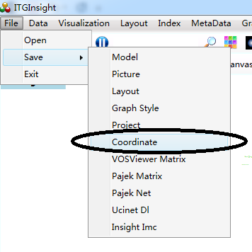
3.30 Export the coordinates 64
3.32 Draw all visual graphics into Word at once 65
3.34 Saving vector graphics in SVG format 67
4.1 Network Graph Clustering Analysis 69
4.2 Thermal map / topographic map / density map visualization 71
4.3 World Map Visualization 75
4.4 China Map Visualization 75
4.5 Matrix Chart Visualization 75
5.1 Use filters to switch analysis objects 77
5.2 Analysis threshold, parameter setting 78
5.5 Name dictionary setting 82
5.6 Company dictionary setting 82
5.7 Country name dictionary setting 83
5.8 Provincial dictionary setting 83
5.9 Dictionary content case sensitivity setting 83
5.10 Apply regular expressions in dictionaries for advanced filtering and replacement 84
5.11 How to set the dictionary when using the software for the first time 85
6.1 Select the data source to be washed 86
6.3 Data manual grouping to achieve data cleaning 87
6.4 Automatic data grouping for data cleaning 88
6.6 Use the dictionary to clean the data again, data analysis, automatic grouping 90
6.7 Save the cleaning result 90
6.8 Combined analysis (cross-dimensional, cross-level co-occurrence matrix, citation matrix) 91
6.9 Grouping statistics (after data cleaning, statistics shall be made according to new groups) 93
6.12 Convert Dataset to Excel or TXT 98
6.14 Convert Dataset to Itgn File 99
Chapter 7: Auxiliary Software Tools 100
7.1 INPADOC family patent visualization analysis tool 100
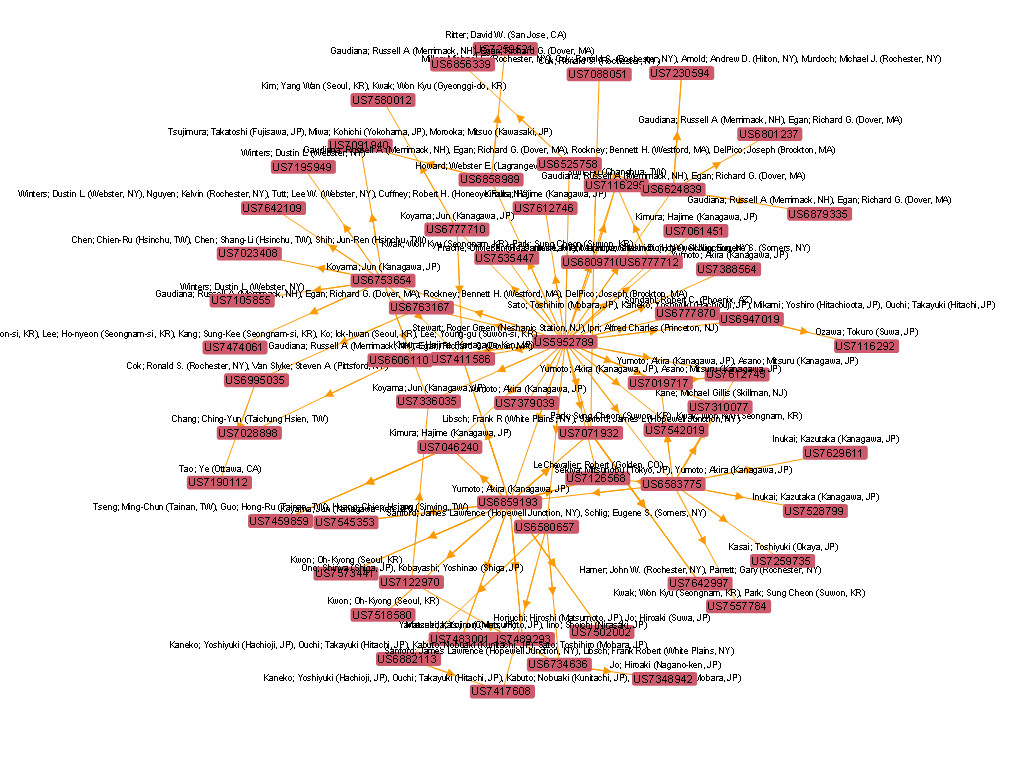
7.2 US Patent Citation Visualization Analysis Tool 100
7.3 US Patent Claim Analysis Tool 101
Chapter 8: Custom Structured Data Visualization 103
8.5 Excel format data (universal format) 105
Chapter 9: Recognition of Chinese and English Technical Terms (Building User-Defined Thesaurus) 108
Chapter 10: Interacting with VosViewer, Pajek, Ucinet 109
Chapter 11: Automatic Reporting 111
12.1 Metadata Import and Export 113
Chapter 13: Converting to References 115
13.1 Export literature to WORD in bibliographic format 115
Appendix A. Co-author/co-occurrence/coupling 116
Appendix B. Correspondence 117
Appendix D. Citation relationship 118
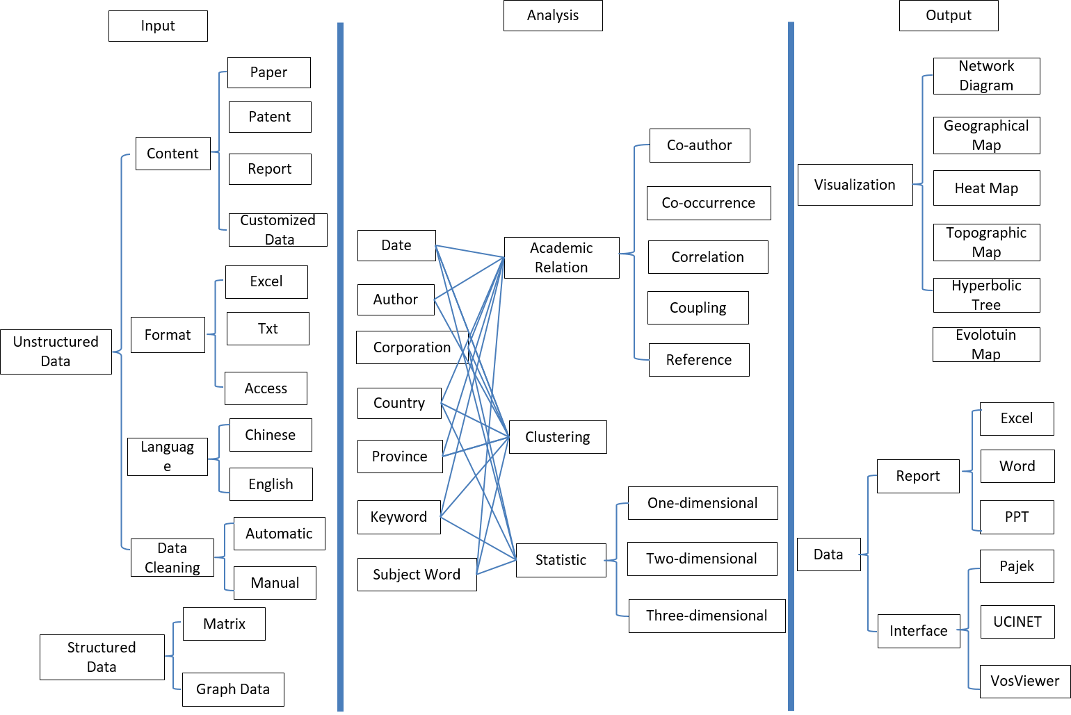
ITGinsight is a text visualization and mining system for general science and technology. This software is a scientific and technological text mining and visualization analysis tool designed primarily for analyzing and visualizing scientific and technological texts, such as patents, papers, reports, and newspapers. It can also be used to analyze internet text data, such as Weibo and WeChat. The visual mining methods available include collaboration relationship visualization, co-occurrence relationship visualization, coupling relationship visualization, association relationship visualization, citation relationship visualization, and evolution analysis visualization. The visualization output options include network diagrams, heat maps, density maps, world maps, matrix maps, evolution maps, and cluster diagrams. This tool enhances the processing of large-scale data by integrating cluster analysis, technical heat maps, technical topographic maps, and technical weather maps into the system.
This tool enables users to visually mine a wide range of scientific and technological texts, including data from SCI, CNKI, Wanfang papers, Derwent patents, US patents, Chinese patents, and European patents. It can also support scientific research management tasks, such as academic evaluation, technology monitoring, technology opportunity analysis, and competitive situation analysis, as well as intelligence analysis tasks. Additionally, the tool serves as a comprehensive intelligence analysis platform that provides basic dimensional statistics, Excel reports, Word intelligent reports, and PPT visual output in addition to text mining and visual analysis.
The system supports any text and graphic data in a user-defined format and offers data and use interfaces with intelligence analysis tools such as Vosviewer, Pajek, and Ucinet for complex network analysis.
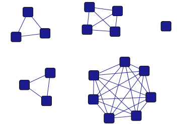
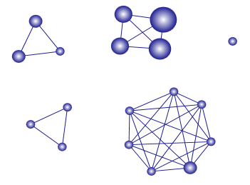
The functional framework of the system can refer to the following two figures. For the specific operation process, see Chapters 3 and 4.
1.3 Comparison of similar tools
| Serial number | software | Attribution | Function type | analyze data | Analytical method | Visual input | Automatic report | ||||||||||
| data source | type of data | Data cleaning | User vocabulary | Basic statistics | Cooperate | Coocurence | Citation | Correlation | evolution | Visual graphics | Interactive interface | Automatic report | Automatic report | ||||
| 1 | UCNET | United States
University of California |
Visual display tool | Arbitrarily | structure | no | no | no | no | no | no | no | no | Statistical chart, network diagram | weak | no | no |
| 2 | Pajak | Slovenia
Ljubljana University |
Visual display tool | Arbitrarily | structure | no | no | no | no | no | no | no | no | Network diagram, tree diagram | strong | no | no |
| 3 | Vxinsight | United States
Sandia National Laboratory |
Visual display tool | Arbitrarily | structure | no | no | no | no | no | no | no | no | Network diagram, theme map | strong | no | no |
| 4 | CiteSpace | United States
Drexel University Chen Chaomei |
Text-based visual analysis software | Arbitrarily | Structure/non-structure | Have | no | no | Have | Have | Have | no | no | Network map, map | strong | no | no |
| 5 | True-Teller | Japan
Nomura Research Institute |
Text-based visual analysis software | Arbitrarily | Structure/non-structure | Have | no | no | no | Have | no | no | no | Thermal map, network map | weak | no | no |
| 6 | VosViewer | Netherlands
Center for Science and Technology Research, Leiden University |
Text-based visual analysis software | Arbitrarily | Structure/non-structure | Have | no | no | Have | Have | no | no | no | Thermal map, network map, cluster map | weak | no | no |
| 7 | Vantage-Point | United States
GIT Technology Policy and Assessment Center |
Text-based visual analysis software | Arbitrarily | Structure/non-structure | Have | Have | Have | Have | Have | no | Have | no | Statistical chart, matrix chart, network diagram | strong | Have | Have |
| 8 | Thomson Data Analyzer | United States
Thomson Reuters |
Text-based visual analysis software | Arbitrarily | Structure/non-structure | Have | Have | Strong | Have | Have | no | Have | no | Statistical chart, matrix chart | strong | Have | Have |
| 9 | ItgInsight | China | Text-based visual analysis software | Arbitrarily | Structure/non-structure | Have | Have | Strong | Have | Have | Have | Have | Have | Thermal diagram, network diagram, matrix diagram, cluster diagram, evolution diagram, hyperbolic tree | strong | Have | Have |
1.4 Technical Advantages of ITGInsight Compared to Benchmark International Products
ITGInsight excels in terminology recognition, Chinese language support, data processing capacity, and aesthetics of visual display, making it the preferred choice for users in China. In comparison to other products, ITGInsight has a more extensive data processing capacity, making it an ideal solution for users dealing with large volumes of data. Moreover, ITGInsight’s visual display is designed to be more aesthetically pleasing, resulting in a more user-friendly experience. Overall, ITGInsight’s technical advantages make it a valuable tool for users seeking advanced text mining and visual analysis capabilities.
- University Library
- Institute of Science and Technology Information
- Enterprise engineering technician
- Enterprise Intellectual Property Management Decision-Maker
- Universities, research institutions, teachers, students
- Other intelligence analysts, intellectual property analysts, consultants, agents, law firms
The software is available in four different versions, namely the secure version, enterprise version, teaching version (research version), and student version (community version). The student version can be downloaded from www.itginsight.com and does not require registration. It is designed specifically for students to write papers and upload user data without technical support. The other versions are for paying users.
The software is available in both 32-bit and 64-bit versions. An ordinary computer with a 64-bit version and 8GB memory can support at least 100,000 pieces of data analysis/cleaning, while a 16GB memory can support at least 150,000 pieces of data analysis/cleaning. In actual use, users with 256GB memory and 24-core CPU can handle more than 5 million documents.
For text clustering analysis, an ordinary computer with 8GB memory can support clustering of 20,000 patents or papers. However, improving the computer configuration can increase the number of clustered patents or papers
1.8 Video Tutorials and Technical Support
This software offers detailed video tutorials available at http://cn.itginsight.com/course/.
Technical support is available based on user level. Online technical support can be accessed via QQ: 3593374821
For enterprise-level users with the highest authority, on-site technical support and training are also provided.
1.9 New Features in Previous Versions
The new features in V2.3.0 include:
- Changing from integers to floating-point numbers for edges
- Automatic reporting feature, adding WeChat Pay for personal users
- Community version and student version have opened temporary authorization and increased data analysis limits through WeChat Pay
- Adding vector graphics
- Fixing a bug in the Dataset where the use of a vocabulary list during data reading did not remove duplicates, resulting in differences in the statistics of first, second, and third authors.
The new features of V2.2.0 are as follows:
- Enhance visualization of project coupling and project citation relationships.
- Include a menu bar, visualization, transfer to ITGN, and group statistics on the dataset page.
- There are four dictionary processing methods commonly used in data analysis. The methods include word list + word segmentation and word segmentation + dictionary. The choice between these methods primarily depends on the word list settings. The word list can be modified through deletion, replacement, regular replacement, or addition (user-defined word extraction).
- Data cleaning section: The word segmentation and word list should be standardized to the same format in the background. The specific method will depend on the content of the word list.
- Bug fix: The lack of ordering in provinces can lead to inaccurate sorting of cooperation analysis, and Doc To Excel does not provide sorting capabilities.
- Two filters, Wos5 and Wos6, have been added to extract authors and institutions with addresses. Additionally, SCI ‘s institutional dictionary allows for multiple replacements.
- This means that an organization can be replaced with more than two new organization names in the order specified by the new organization names in the dictionary.
- The dataset now includes communication authors, institutions, countries, as well as their corresponding grouping, statistics, and clustering.
The new functions added in V2.1.0.0 are as follows:
- The addition of a breakthrough analysis feature.
- The inclusion of an SCI/SSCI secondary unit filter.
- The addition of grouping statistics for data cleaning.
- The addition of “Doc To Excel” and “Doc To Txt” functions on the dataset page, and revision of the 2Excel method for data cleaning and reading, resulting in faster processing speeds.
- The addition of a big dataset and SQLite mode, allowing for processing of millions of data points on a single computer.
- Semantic fingerprinting and quick data cleaning have been added for authors, organizations, and keywords.
- Node name modification now supports multiple regular expression replacements.
- A combined query feature has been added for querying dataset data.
- Batch replacement of node names is now possible, and regular expressions have been added to support this.
- Automatic grouping and batch replacement using regular expressions have also been added.
The new features of V2.0.0.1 are as follows:
- Enhanced light and dark mode appearance.
- Fixed bug causing suspended animation in progress bar.
- Added a ToReference function, enabling conversion of bibliographic items into reference analysis format.
- Resolved the issue of incomplete mod file format when saving evolution maps.
- Added the option to output combined analysis results in txt format to avoid compatibility issues with Excel installations.
- Introduced a new Recluster function.
- Included the ability to modify node grouping and clustering.
- Enhance technical competitiveness indicators
- While performing data cleaning, include read-only settings for the first author, first unit, and first country
- Integrate the data cleaning and metadata pages into the main page
- Add word segmentation to all four modes in the data cleaning process
- Improve the interaction between the cluster diagram and the dataset by adding the label modification ReTag function
- Introduce K-means clustering with N clusters
- Implement automatic labeling of clustering results
- Improve data cleaning performance by increasing the amount of data read and reducing read time by over 50 times, and increase the speed of automatic grouping by over 5 times
- Enhance dimensionality reduction capabilities by including PCA and KPCA techniques.
The new features of V1.9.1.0 are as follows:
- The dictionary now includes additional modes, such as uppercase, lowercase, mixed case, capitalization, and regular expression filtering.
- The calculation of betweenness centrality has been revised for greater accuracy.
- The software now supports Chinese and English mixed data analysis, with separate word length thresholds for Chinese and English.
- The operation of shortcut keys has been enhanced for greater efficiency.
- The software now features optimized data reading speed, resulting in a 40% increase in performance when working with large-scale data and dictionaries.
- A clustering thematic topographic map has been added to provide more detailed and comprehensive analysis.
- The graph density indicator has been increased to improve data interpretation.
- All English words are now treated as singular, and a regular expression replacement function has been added to simplify vocabulary management.
- The software now supports Scopus data, expanding the range of available data sources.
- The world map and China map now have a transparent background, and the coordinate layout has been retained while the map layout of China provinces has been removed.
- A new feature has been added to display the number of user logins as a group prompt.
- The data cleaning feature has been fixed to remove extra spaces in Chinese grouping.
The new features of V1.9.0.0 are as follows:
- A legend has been added to the software, and users can draw a legend in PPT to improve the visual presentation of their data.
- The filter feature now supports merging multiple summary and keyword fields, with users able to split them using the “|” character.
- The automatic report feature now supports Patsnap, Incopat, and Innovation data sources, providing users with more options for data analysis.
- The tables in the automatic report feature are now centered to improve their readability and presentation.
- When the data time field is missing, the software will remove the 1900 data from the visualization to ensure accurate and reliable analysis.
- The software now includes improved filtering for highly cited papers and patents, with users able to set Number1, Number2, and Number3 thresholds to filter data. This feature will only analyze and clean the data that exceeds these thresholds.
- The software now includes an automatic analysis report template for single institution literature data, as well as an automatic report analysis template for comparative analysis of literature from multiple institutions.
- The dictionary now features a reverse filtering function, which enables users to analyze only the names, institutions, countries, provinces, categories, and keywords contained within the vocabulary.
- A new drawing robot operation has been added to enable users to draw all visual graphics at once, improving the efficiency of data visualization.
- The software now includes a progress prompt in the status bar when automatically grouping parts, providing users with real-time feedback on the progress of their analysis.
The new features of V1.8.0.0 are as follows:
- The software now includes Class 3 and Class 4 options for improved data classification and analysis.
- The automatic report engine has been optimized for improved performance and efficiency, with improvements made to the correlation analysis part and report template component composition.
- The aiReview.online and SciReport.online services are now available to users, providing additional resources and support for data analysis and reporting.
The new features of V1.7.0.0 are as follows:
- The software now includes project co-author analysis for improved collaboration tracking and analysis.
- The analysis part has been updated to remove processing operations related to outliers, streamlining the data analysis process.
- A new single IP reminder function has been added, providing users with a notification when a single IP is used for multiple logins.
- The LinLog layout has been added and set as the preferred layout for improved data visualization.
- The automatic report feature has been upgraded to be fully automatic, with a separate system called ezReport created to provide users with independent authority and improved reporting capabilities.
- The software now includes default parameter optimization settings and background calculation for improved performance and efficiency.
- The summary field in the filter now supports multiple field merging, with the “|” symbol used to split and analyze multiple fields at once.
The new features of V1.6.0.0 are as follows:
- A new metadata function has been added, similar to the addition of GELPHI columns. This allows for improved data organization and analysis.
- Six new presentation forms of theme maps have been added, similar to the theme maps found in VOSViewer. This provides users with additional visualization options.
- A new cluster density map has been added, improving the analysis and visualization of clustered data.
- A label anti-overlapping function has been added to improve the readability and clarity of visualized data.
- The node size contrast parameter sizevariation has been increased, allowing for improved size contrast between different nodes in the data.
- Increase the panel border size setting, with the purpose of intercepting density maps, heat maps, cluster maps, and all other graphics.
- Added the direct export function of coordinates.
- Added the function of data link, i.e., the addition of the “Go To Related” function in the data cleaning module.
- Added the TSNE layout.
- Added floating windows.
The new features of V1.5.0.9 are as follows:
- Added a new function for batch modification of node sizes.
- Added a high-definition screenshot function for regular computers.
- Increased the automatic report function for SCI papers.
- The software is now available in different editions including student, academic, teaching, enterprise, group user, and military editions.
- Added a batch function to “show or hide node names”.
- Fixed a bug causing forced exit due to configuration file errors.
- Users can now customize density map colors.
- Added automatic reports and user manuals in English.
The new features of V1.5 are as follows:
- Added 3D statistical analysis
- Added document clustering and density map visualization after data cleaning
- New smart reporting feature
- Added “docadapter” mode to read data without analysis and analyze after reading docadapter again
- Increased coverage of the convex hull in the network graph
- Added registration-free function for group customers
- Added support for processing .netx format files
- Increased the option to flip graphics horizontally and vertically
- Added visualization of frequency matrix, similarity matrix, and Pearson matrix in Excel format
The new features of V1.3 are as follows:
- New theme evolution analysis, tracking the process of technology generation, death, enhancement, weakening, aggregation and fission
- Newly added institutions, authors, countries, provinces, keywords, and technology category evolution analysis to expand the scope of subject evolution analysis
- Add SPC main path indicators to identify key technical nodes in the process of technological development
- Add computer recognition of the same name with different fingers and different names with the same finger
The new features of V1.2 are as follows:
- A brand new report engine is introduced, enabling users to generate nearly 100 analysis reports with just one click, providing a comprehensive understanding of the data characteristics.
- The semantic analysis function is enhanced, allowing for automatic identification of similar subject words, organization names, personal names, and geographical names.
- The intelligent combination analysis feature enables visualization of cross-dimensional and cross-level data matrices, providing deeper insights into the data.
- The rendering technology is optimized, with the addition of technology cloud maps, knowledge diffusion maps, efficiency matrices, and maps of Chinese provinces.
Chapter 2: Installation and operation
2.1 Installation prerequisites
Operating system
Windows 7 or later, with Office 2010 or later installed. The 32-bit software version is compatible with the 32-bit version of Office, and the 64-bit software version is compatible with the 64-bit Office.
Hardware configuration
Memory: 1GB or more; Hard disk: 100MB or more; CPU: Main frequency of 1GHz or more.
If NetFramework4.5 is not already installed, download and install it from the network. The system will automatically download it without the user having to do specific operations.
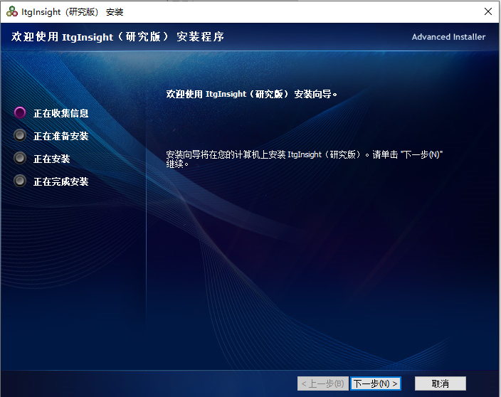
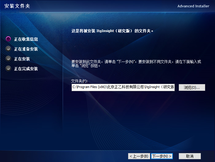
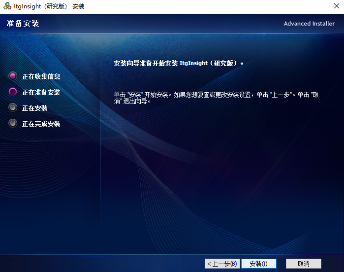
The ITGInsight green version does not require installation. Simply decompress the file and run the .exe file directly. For the non-green version, you will need to install it by clicking on the setup.exe file in the installation folder. The following dialog box will appear insequence:

To uninstall the green version, you can delete the folder directly. For the non-green version, open the “Control Panel,” select “Add or Remove Programs” or “Programs and Features,” and find ITGInsight in the list of current programs. Then, click on the “Uninstall” button.
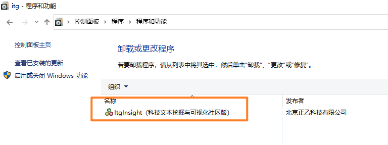
Click the “Delete” button.
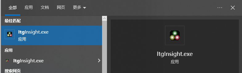
After installation, the system’s startup shortcuts will be placed on both the desktop and in the program folder, as shown below:
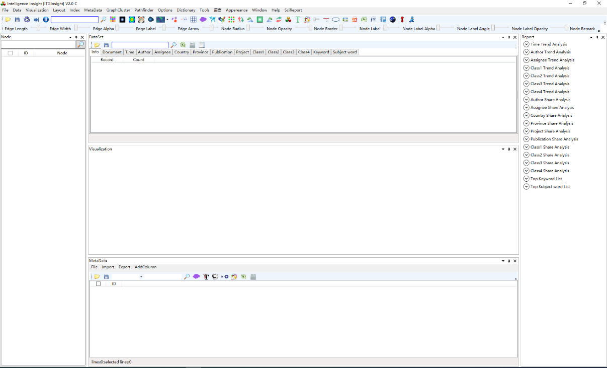
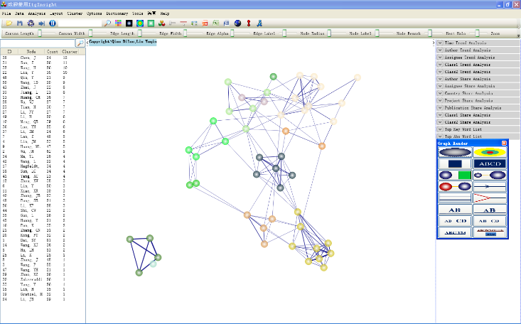
After starting the software, the main window is composed of the visualization area, dataset area, metadata area, node area, and report area, as shown in the figure below. By default, only the visualization area, node area, and report area are displayed. However, you can configure the display settings for each area by using the Window/Window button in the menu bar.
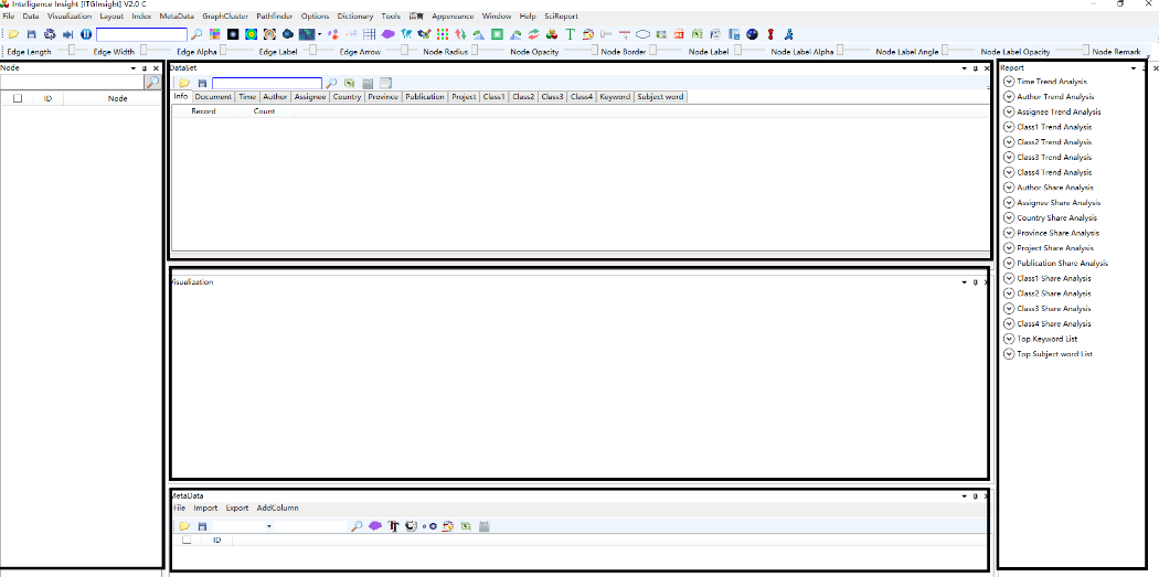
The software supports both light and dark appearances, which can be switched through the Appearance button in the menu bar. The dark and light appearances are shown in the figure below.

In most cases, the system requires both local and network registration. However, if the software starts normally, local registration is already complete, and only network registration is necessary. Commercial users generally do not need to complete local registration.
2.5.1 Local Registration Method
To complete local registration, follow these steps:
1)Run the HID.exe file located in the hid subdirectory of the software installation directory to obtain the computer’s serial number. 
2)Send the machine code along with the institution, user, and email address to the customer service mailbox.
3)Once the registration information has been received and verified, the customer service team will send the time-limited authorization file to the user’s email address. The time limit is typically set to one month. If you require an extension to the time limit, you must request one.
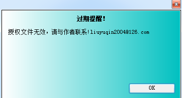
Users who have not completed local registration will periodically receive an “Authorization Warning” window when using the software, as shown below:
4)Our software technology support QQ group (198853346) will publish a universal local registration file every three months. The authorization is not bound to the computer hardware, and any user can complete local registration.
2.5.2 Network Registration Method
To complete network registration, follow these steps:
Complete local registration as described above.
Run the software and click Help > Register to bring up the following screen: 
Send the machine code along with the institution, user, and email address to the customer service mailbox. The customer service team will complete the network registration on behalf of the user. Users who have not completed network registration will be automatically logged out after 5 minutes.
2.5.3 Group customer registration
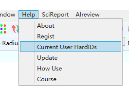
Group customers do not require network or local registration. However, if the number of simultaneous login users exceeds the number of group purchases, the software will display the total number of currently logged-in users when it is launched. For instance, if a group has purchased 5 accounts, only 5 users can be guaranteed to be online at the same time. When a group user attempts to log in, the login status will be verified. If the user limit has been reached, the system will notify the user that the maximum limit has been reached and display the hardware ID of the logged-in user. The current user can forcibly log out the hardware ID of the logged-in user. Otherwise, if the current user logs in, they will also be automatically logged out due to reaching the user limit. After a group user logs in, they can view the hardware IDs of all logged-in users through the help function, as shown in the figure below.

2.5.4 Confidential version registration
The confidential version of ITGInsight necessitates local registration and prohibits network registration. One code can only be used on one machine, and the software cannot be connected to the internet. This version is best suited for data-sensitive or confidentially qualified units. If the confidential version is connected to the internet, it will be automatically shut down.
To upgrade ITGInsight, click on “help” -> “update.” In a networked environment, the system will automatically check for the latest software version and upgrade the system. It is crucial to ensure that ITGInsight is closed during the upgrade process.
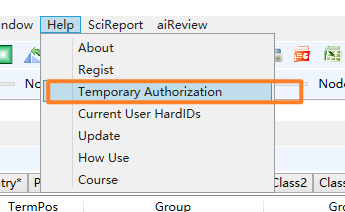
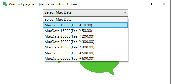
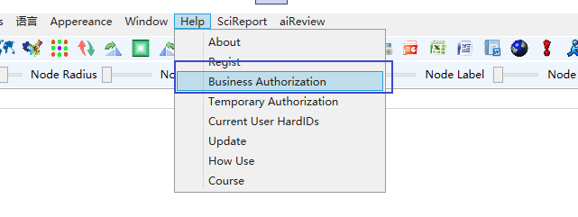
For Community/Student edition users, there are limits on the amount of data analysis that can be performed. However, users can increase the data analysis limit by clicking on “Help” and then selecting “Temporary Authorization”, which allows them to make a payment via WeChat. The temporary authorization is valid for 1 hour, during which time data analysis and cleaning can be performed according to the relevant payment amount.
Enterprise and research edition users can download the authorization file through commercial licensing, and do not need to copy the authorization file again after each software upgrade or when installing on a new computer. To authorize the software, click on “Help” in the software toolbar, then select “Commercial Licensing”, and enter the username and password provided at the time of purchase. Please run the software as an administrator when using it.

Chapter 3: Data Analysis and Visualization
3.1 Data format conversion / reading of document data to generate itgn files
The initial step in utilizing ITGInsight for data analysis is to convert the literature data into the ITGInsight data format, followed by applying the data conversion function to analyze the data.
To access the data conversion page, click on “Data/Data->Analysis/Analysis” on the menu bar, as illustrated below:

Click on the “File” tab under the “Data Analysis” tab. ![]() ,Pop up the data navigation dialog box, select the data source, as shown below:
,Pop up the data navigation dialog box, select the data source, as shown below:

The system supports several types of data for analysis, including Chinese core journal data downloaded from CNKI (refer to example_data_cnki.txt in the installation directory), SCI paper data and Derwent patent data downloaded from Web Of Science (refer to example_data_wos.txt in the installation directory), and patent analysis software ItgMining for the exported patent data (refer to the sample data such as example_data_itgmining.xls or example_data_itgmining.accdb in the installation directory). The data file can be in Excel03, 07 and above, Access03, 07 and above, or txt format. Additionally, the data file can also be in the docapadter format, which is a data file generated by ITGInsight.
At “Filter”, click ![]() ,Pop up the filter and select the navigation dialog box, select the filter, as shown below:
,Pop up the filter and select the navigation dialog box, select the filter, as shown below:

Choose a filter from the dropdown list. For instance, if the data is exported by ItgMining, select the “filter-itgmining” filter so that the system can identify the data source and apply the corresponding data processing rules. If the data is from SCI, select the “filter-wos” filter.
Enter the delimiter in the “Segment/Delimiter” column. By default, the system uses “;”. If there are multiple delimiters, enter them all.
If a record of an object to be analyzed contains multiple records, such as “author”, and a database record has multiple authors separated by “;”, the system will recognize all authors by using “;” as the separator during the analysis.
If the selected data is in txt format, the “Encoder/Encoding” column is functional, and the system parses the text based on the encoded content. If the encoder setting is different from the actual encoding of the data txt, the system may not be able to analyze the text content accurately. You can select the “Encoder/Encoding” setting from the dropdown list or manually enter it.
“Save” column, click ![]() ,Fill in the path and file name of the file save. The system defaults itgn to the file suffix. This file is the project file for visual analysis.
,Fill in the path and file name of the file save. The system defaults itgn to the file suffix. This file is the project file for visual analysis.
Under the “Statistic” tab, you can select the dimension of the statistical analysis. One-dimensional statistics are mandatory and two-dimensional statistics are optional. When selecting subsequent association analysis, two-dimensional statistics automatically become mandatory. Selecting two-dimensional statistics will increase the analysis time.
In the “Analysis/Analysis” tab, you can select the content of the analysis to be performed, such as “Coauthor/Co-Occurrence Analysis”, “Correlation/Correlation Analysis”, “Correspondence/Correspondence Analysis”, “Reference/Citation Analysis”, etc. Multiple options are available.
You can set the start and end time of the analyzed data in the “Time” tab.
Under the “How many/How many” tab, you can enter the number of institutions, authors, countries, categories, journals, keywords, and digest words to be analyzed, as well as the number of analyses to be performed.
Finally, switch to the “Dictionary” tab, as shown below:

Select the dictionary, the first time users can find the relevant dictionary file in the dic directory of the software installation directory.
Switch to the Alpha tab, as shown below:
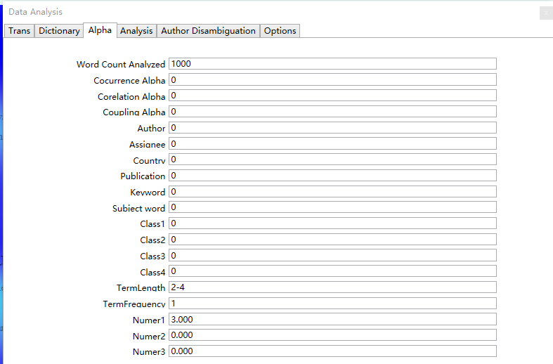
For first-time users, it is recommended to save the default settings unchanged. Among them, TermLength and TermFrequency represent the word length and word frequency limit for extracted keywords. For English, the recommended word length is 2, and for Chinese, it is 3. When the amount of data is relatively large, increasing the word frequency threshold can speed up the analysis.
Regarding the Threshold setting for Number1, taking SCI papers as an example, when Number1 is set to 3, only papers with more than 3 citations will participate in the analysis, while papers with 3 or less citations will be filtered out and excluded from the analysis. Similar thresholds can be set for Number2 and Number3, but it is recommended to set them to 0.
To proceed, switch to the Analysis tab, as shown below:
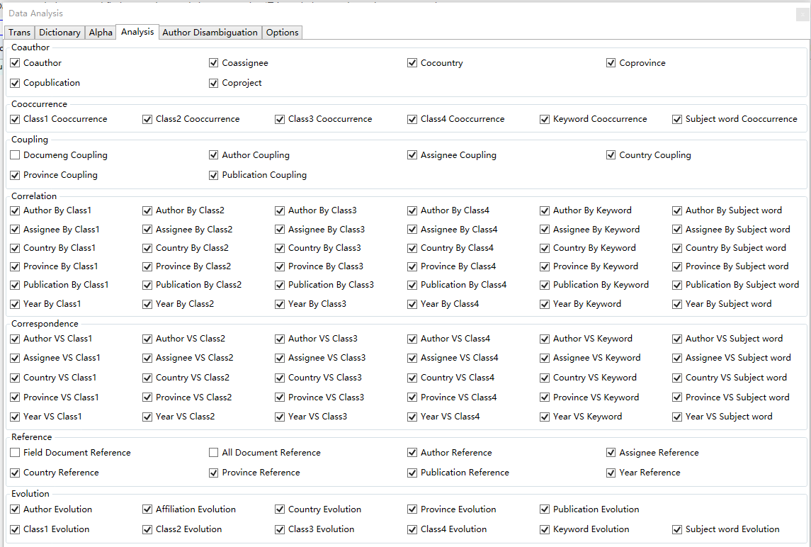
The first use remains the same as the default setting. However, when dealing with a large amount of data, performing Document Reference/Document Citation Analysis can take a long time. Therefore, it is recommended to remove irrelevant items to speed up the analysis process.
Author Disambiguation/author disambiguation label is as follows:

If the same name appears multiple times in the dataset, it can be difficult to determine whether the records refer to the same person or different individuals. By default, the system assumes that all instances of the name refer to the same person. However, selecting the Assignee/Institution option can help to disambiguate authors by considering the institutional information associated with each document. Other field selections may provide similar benefits in terms of disambiguation.
Switch to the Options/Options tab as shown below:

The ‘Save Document Adapter’ feature allows you to retain the intermediate analysis result after reading the data, which is saved with *.docadapter suffix. This file can then be used as input for secondary analysis. Similarly, the ‘Apply PFNET’ option enables network graph compression using PFNET during the analysis process. This feature is set to the default option by default.
To finalize the changes, switch to the ‘Trans/Conversion’ tab and click on the ‘OK/Confirm’ button. This will initiate the background data conversion process, which will be reflected in the ‘Main Progress’, ‘Auxiliary Progress’, and ‘Status’ indicators.3.2 Read itgn file for visualization.
To open an ITG project file for analysis, select the ‘File’ menu item on the menu bar or click the ‘Open’ button on the toolbar, as shown below:


This will open the file navigation dialog, where you can navigate to the ITG project file and read it into the system.

After reading the ITG project file, the system displays basic statistics on the right side of the main page, providing some basic dimensional information. To generate visualization results, the visualization area needs to be specified according to the operation mode of 3.3-3.9, as shown below: 
3.3 Coordination visualization
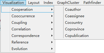
1)Click on the menu bar “Visualization” -> “Cooperation”, as shown below.
2)To access the layout algorithm selection, click on the “Layout” option in the menu bar and then choose from the available options: CR Layout, EV Layout, RF Layout, UP Layout, SP Layout, KK Layout, FR Layout, LL Layout, or VS Layout, as shown below. The selection of the appropriate layout algorithm should be based on the criteria of producing a visually appealing and easily readable graphic. By default, the LL layout algorithm is pre-selected, which is suitable for most visualization scenarios.

3)Click on the toolbar ![]() ,initial visualization analysis graph, as shown below.
,initial visualization analysis graph, as shown below.

3)Click on the toolbar ![]() ,start graphics optimization.
,start graphics optimization.
4)In the graphics optimization process, click on the toolbar ![]() ,stop graphics optimization to get more concise and clear visual analysis results, as shown below.
,stop graphics optimization to get more concise and clear visual analysis results, as shown below.

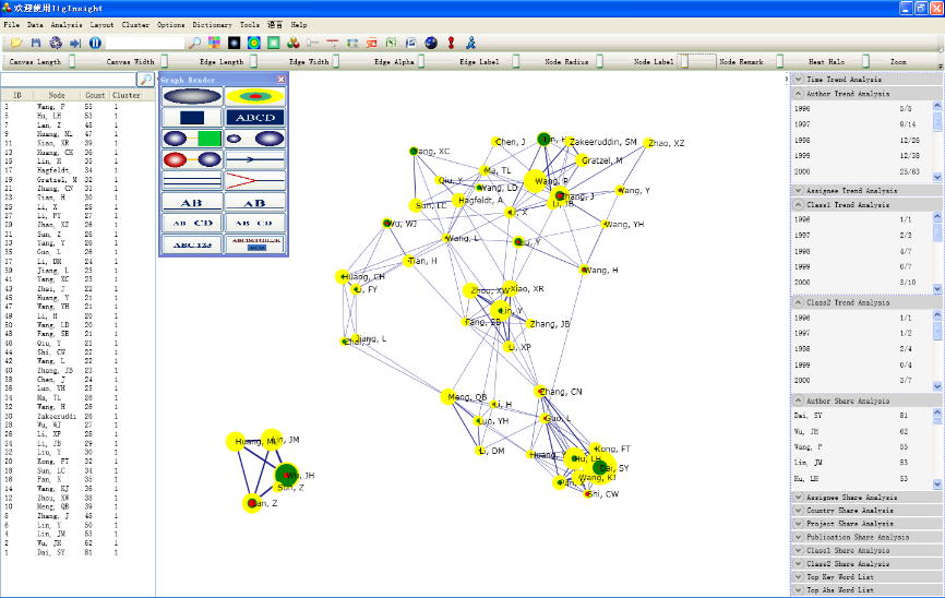
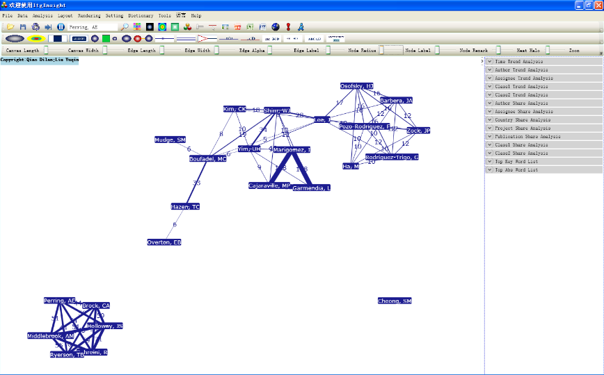
5)To customize the graphics, refer to the “Graphic Style Settings” and “Slider Settings” located at the back of this manual. The following figure showcases a typical visualization of joint relationships, which can be personalized using these settings.
3.4 Visualization of co-occurrence
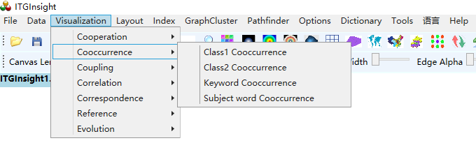
1)Click the menu bar “Visualization/Visualization”——>”Cooccurrence/Cooccurrence Network”——>”Category 1 Co-occurrence/Category 2 Co-occurrence/Keyword Co-occurrence/Abstract Word Co-occurrence”, as shown below.
2)Click the menu bar “Layout/Layout”——>”CR Layout/EV Layout/RF Layout//UP Layout/SP Layout/KK Layout/FR Layout/LL Layout/VS Layout/TS”, as shown below.

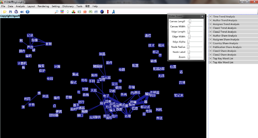
3)The remaining steps for co-occurrence analysis are the same as those for co-author analysis. The following figure displays typical visualization results for co-occurrence analysis.
3.5 Coupling relationship visualization
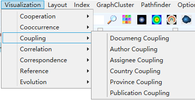
1)Click the menu bar “Visualization/Visualization” -> “Coupling / coupling network” -> “Document coupling / author coupling / institution coupling / country coupling / province coupling / publication coupling”, as shown in the figure below.
2)Click the menu bar “Layout/Layout”——>”CR Layout/EV Layout/RF Layout//UP Layout/SP Layout/KK Layout/FR Layout/LL Layout/VS Layout/TS”, as shown below. 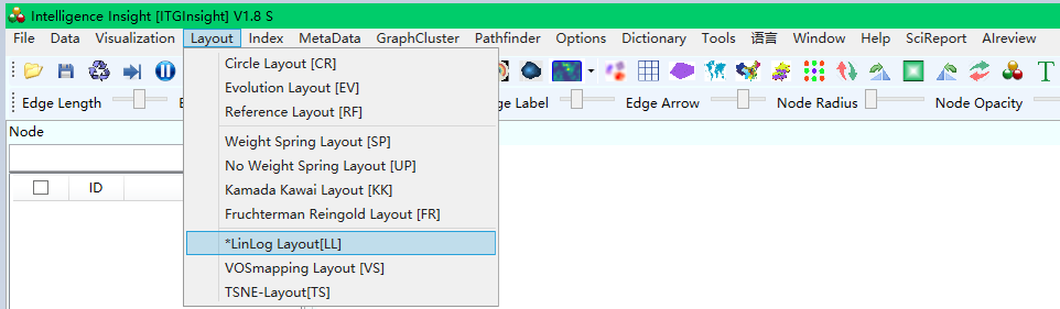
3)The remaining steps for coupled analysis are the same as those for co-author analysis. The following figure displays typical visualization results for coupled analysis.
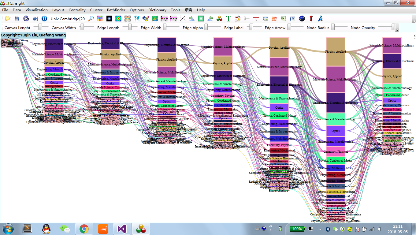
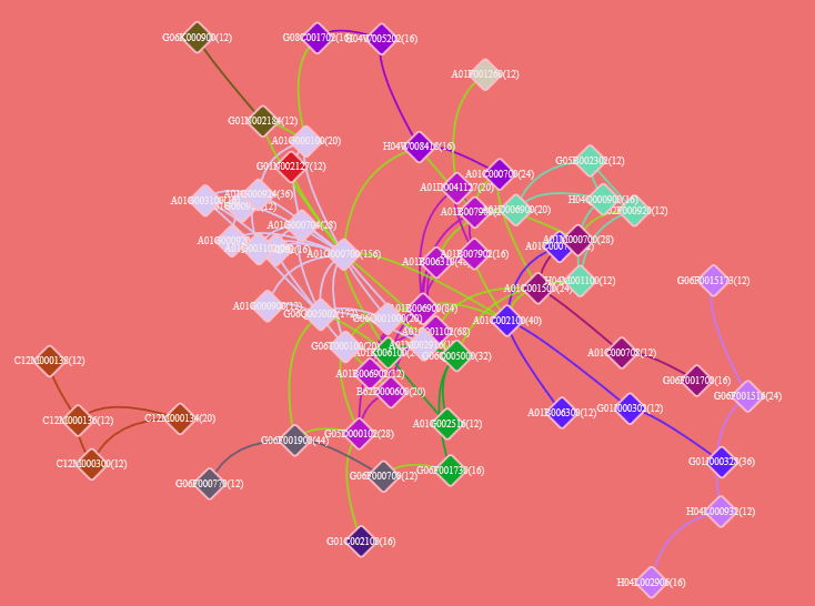
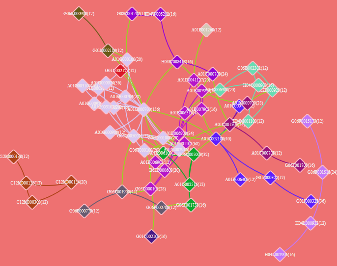
3.6 Association analysis visualization
1)Click the menu bar “Visualization/Visualization” -> “Correlation / Correlation Analysis” -> “Author Association / Institutional Association / Country Association / Province Association / Publication Association / Age Association” -> “Author BY Category 1 / Author BY Category 2 / Author BY Keywords / Author BY Subject Term”; “Institution BY Category 1 / Institution BY Category 2 / Institution BY Keywords / Institution BY Subject Term”; “Country BY Category 1 / Country BY Category 2 / Country BY Keywords/country BY keyword”; “province BY category 1 / province BY category 2 / province BY keyword / province BY keyword”; “publication BY category 1 / publication BY category 2 / publication BY keyword / Publication BY subject word”; “Year BY category 1/Year BY category 2/Year BY keywords/Year BY subject words”, as shown below.

2)Click on the menu bar “Layout” -> “UP layout / SP layout / KK layout / FS layout / VS layout”, as shown below.

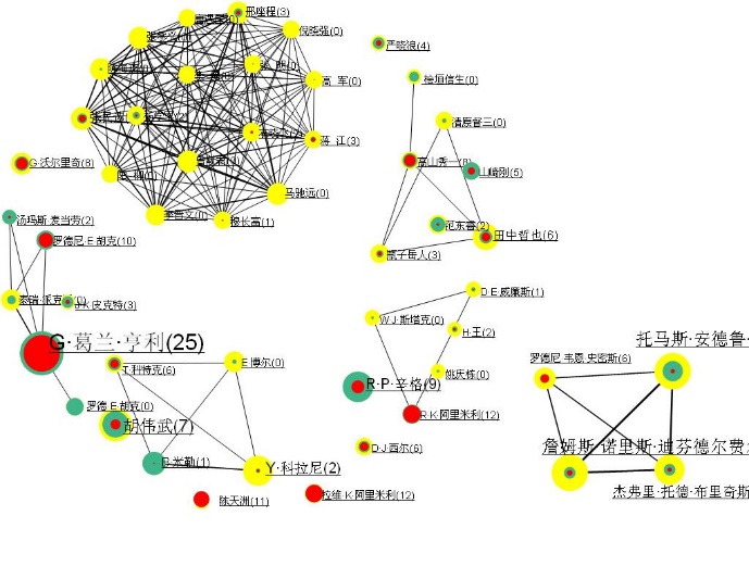
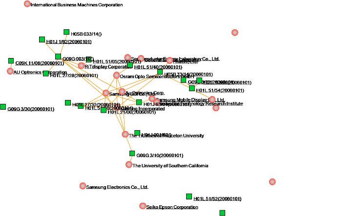
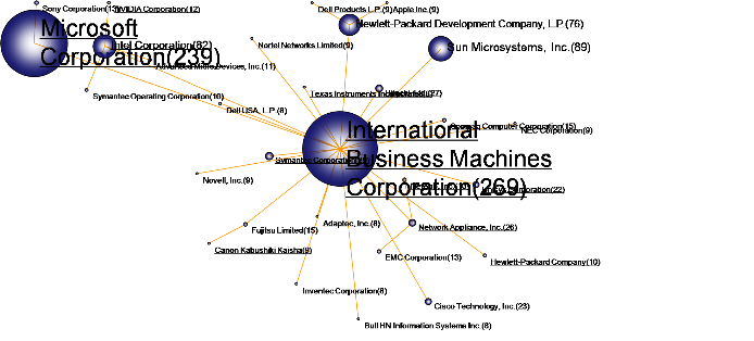
3)The remaining steps for correlation analysis are the same as those for co-author analysis. The following figure displays typical visualization results for correlation analysis.

When conducting time correlation analysis, the RF layout and its corresponding graphics are displayed as shown below.
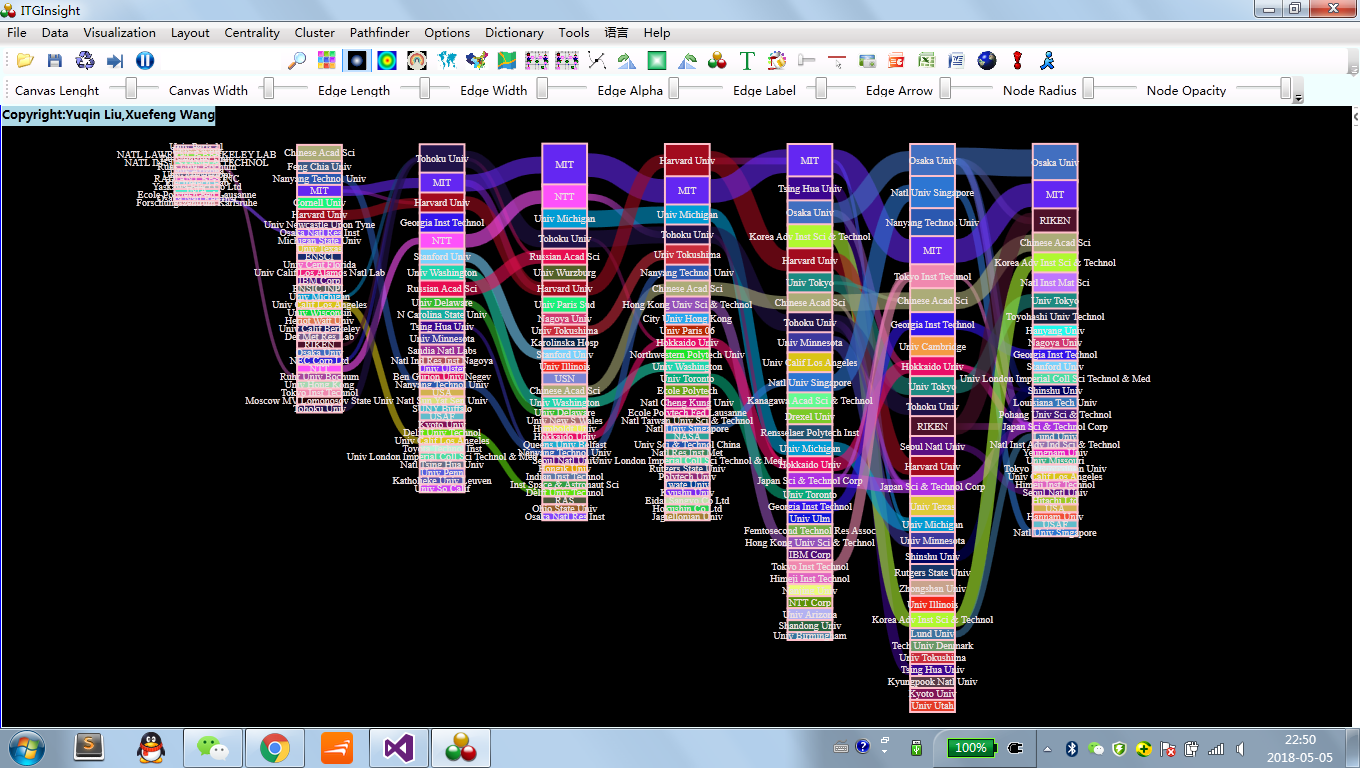
3.7 Correspondence analysis visualization
1)Click on the menu bar “Visualization/Visualization” -> “Correspondence / Correspondence Analysis” -> “Author Correspondence / Institution Correspondence / Country Correspondence / Province Correspondence / Age Correspondence” -> “Author VS Category 1 / Author VS Category 2 Author VS Keywords/Author VS Subject Term”; “Institution VS Category 1/Institution VS Category 2/Institution VS Keywords/Organization VS Subject Term”; “Country VS Category 1/Country VS Category 2/Country VS Keywords/Country VS Subject Term”; “Province VS Category 1/Province VS Category 2/Province VS Keyword/Province VS Subject Term”; “Year VS Category 1/Year VS Category 2/Year VS Keyword/Year VS Subject Term”, as follows Figure.

2)Click the menu bar “Layout/Layout”——>”CR Layout/EV Layout/RF Layout//UP Layout/SP Layout/KK Layout/FR Layout/LL Layout/VS Layout/TS”, as shown below. 
3)The remaining steps are the same as the co-author analysis. The following figure shows the typical visualization results of the corresponding analysis and analysis.

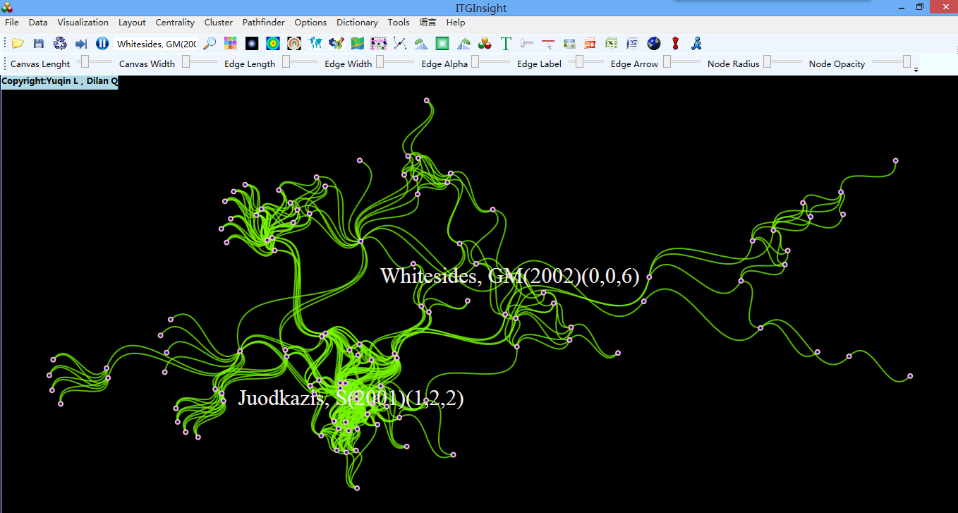
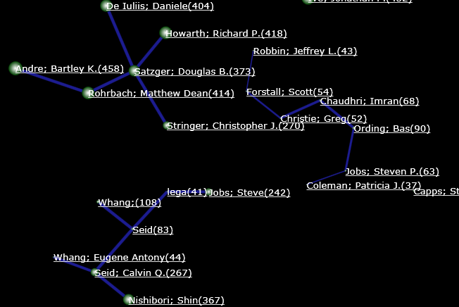
3.8 Citation relationship visualization
 1)Click on the menu bar “Visualization/Visualization”——>”Reference/Citation Analysis”——>”Field Literature Citations/All Literature Citations/Author Citations/Institution Citations/National Citations/Province Citations/Publication Citations/Year Citations”, as follows Figure.
2)Click the menu bar “Layout/Layout”——>”CR Layout/EV Layout/RF Layout//UP Layout/SP Layout/KK Layout/FR Layout/LL Layout/VS Layout/TS”, as shown below.

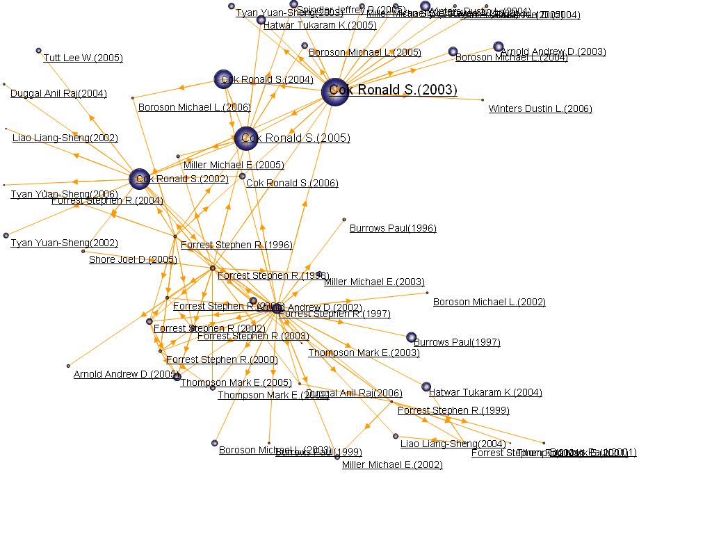
3)The remaining steps for corresponding analysis are the same as those for co-author analysis. The following figure displays typical visualization results for corresponding analysis and analysis.

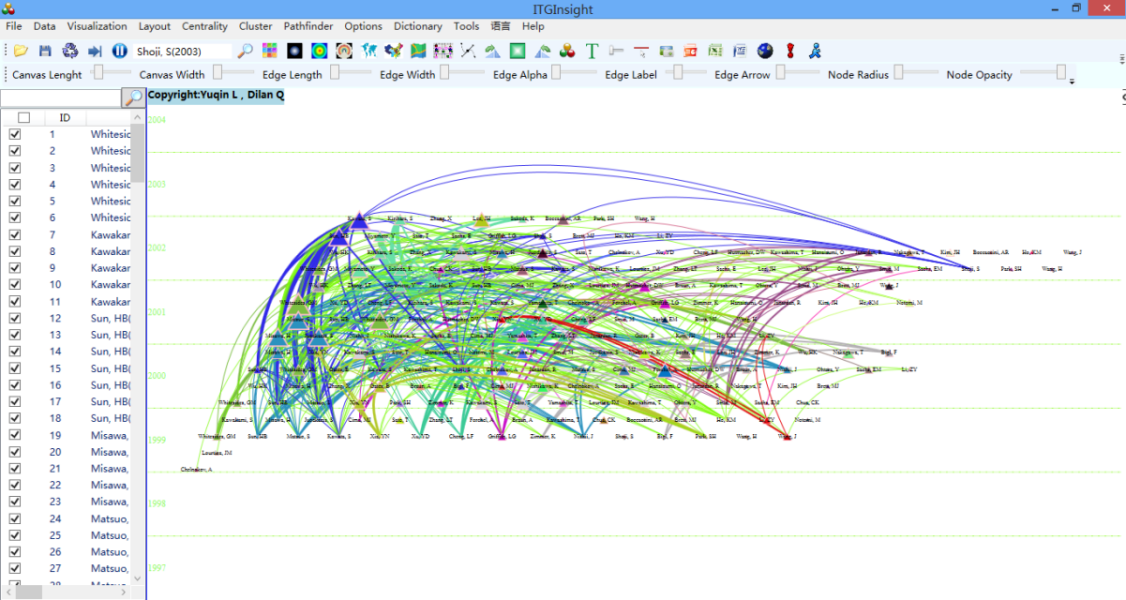
In addition to the network map, citation relationships can also be visualized using the timeline. Click on the RF layout option in the toolbar to display the visual result, as shown below:
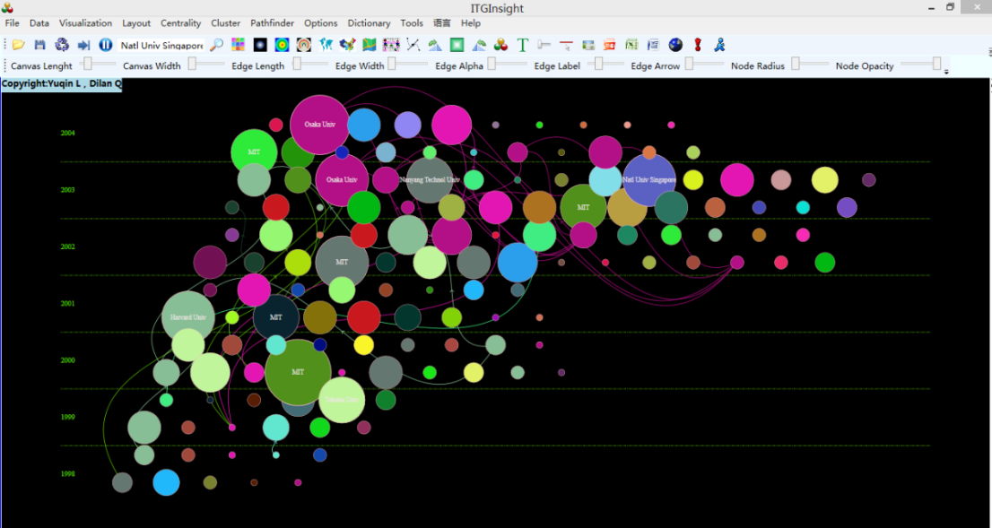
3.9 Evolutionary analysis visualization
Click on the menu bar “Visualization/Visualization”——>”Evolution/Evolution Analysis”——>”Author Evolution/Institution Evolution/National Evolution/Province Evolution/Publication Evolution/Category 1 Evolution/Category 2 Evolution/Keyword Evolution/Topic Word evolution”, as shown below.

The visualization area shows the evolution diagram as follows:

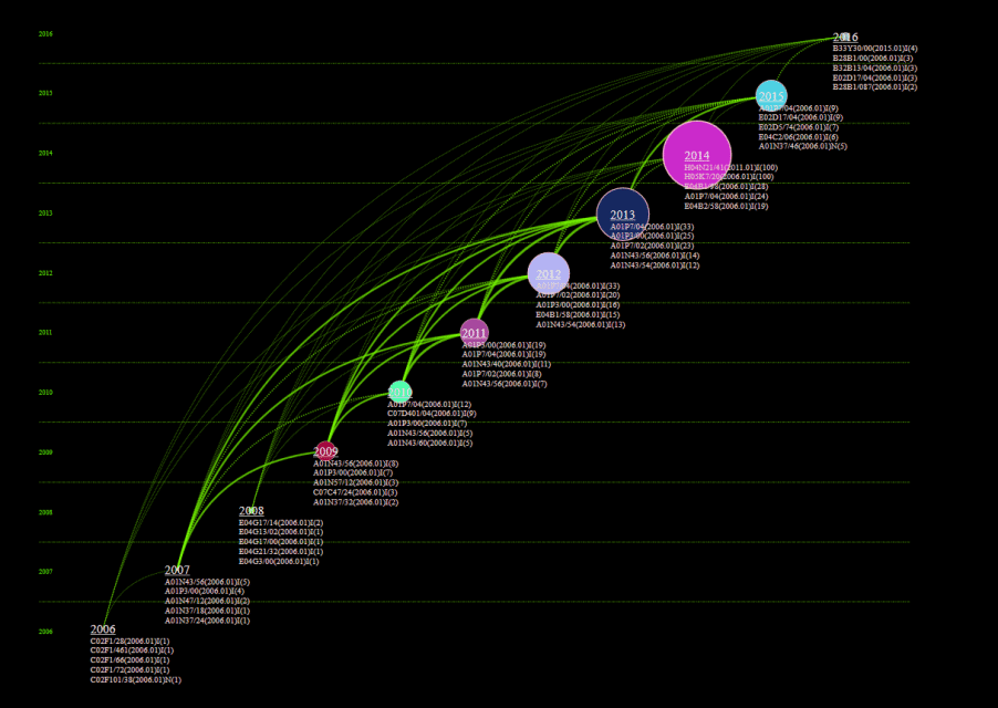
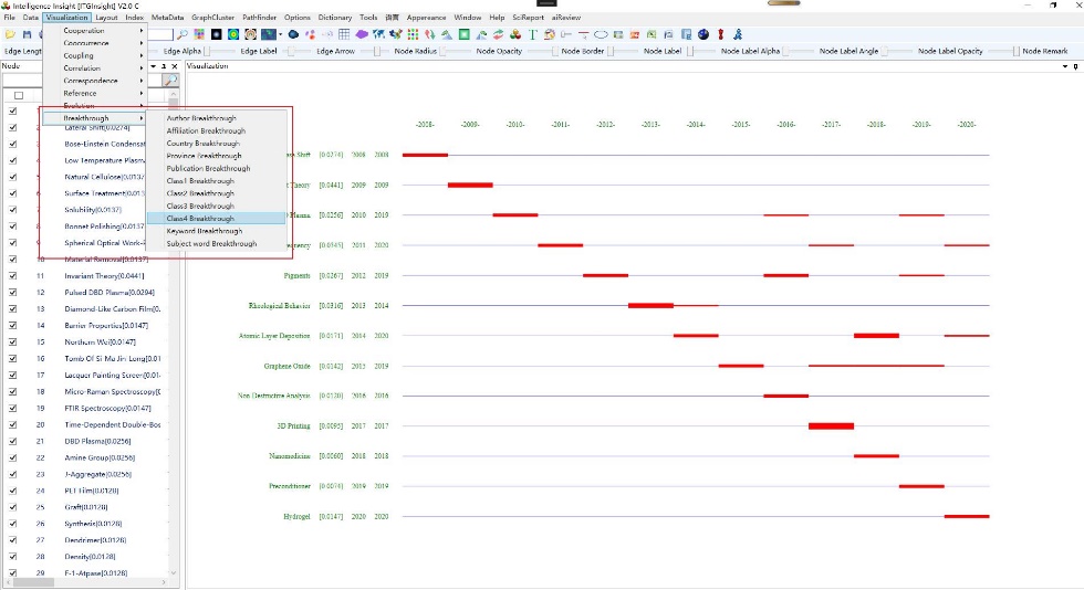
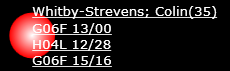
3.10 Breakthrough Analysis Visualization
1) Click on the menu bar “Visualization/可视化” -> “Breakthrough/突破分析” -> “Author Breakthrough/Institution Breakthrough/Country Breakthrough/Province Breakthrough/Publication Breakthrough/Category 1 Breakthrough/Category 2 Breakthrough/Category 3 Breakthrough/Category 4 Breakthrough/Keyword Breakthrough/Subject Breakthrough,” as shown in the figure below.

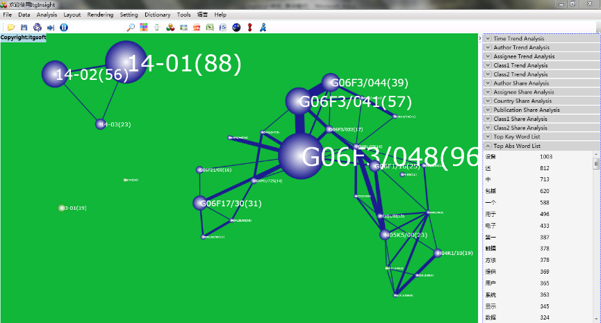
The visualization area displays the evolution graph as shown below, where the values in “[]” represent the breakthrough rate, the red line indicates the appearance in that year, the width can be set to be proportional to the frequency or the same width, and the default is the same width.
3.11 Select an appropriate network layout algorithm to create a visually appealing network map.
During the analysis steps from 3.3 to 3.9, selecting an appropriate layout algorithm is crucial. By default, the layout algorithm generates a network map for the entire visualization area. However, if the algorithm is only applicable to a specific part of the network diagram, users can right-click and hold the Ctrl key while selecting local network nodes by dragging the left mouse button. This allows for different layout algorithms to be applied to different parts of the same network diagram, resulting in a clearer and more readable overall network map. To cancel the local selection, release the Ctrl key and click any left mouse button.
The LL (LinLog) and VS (VosMapping) layout algorithms are different from other algorithms as they position nodes based on the strength or number of relationships between them. In other words, the distance between nodes holds practical significance.
We recommend using the LL (LinLog Layout) algorithm as it satisfies the requirements for most network layouts.
3.12 Key information to filter/delete unimportant cables
During the association analysis process, it’s possible to filter out key information in the multi-network diagram using path compression technology. This involves deleting unimportant connection lines and retaining the relatively important ones. For more details on this, click on PathFinder in the toolbar, as shown below:

There are three compression operations available: Pf(2), Pf(3), and Pf(N-1). These compressions increase in strength gradually. If you want to uncompress, simply press the “Undo” button. However, if you perform two compressions in a row, the “Undo” button will only revert the last compression operation.3.12 Change graphic style / beautify graphics
3.13 change the style of a graphic or beautify a graphic
The graphics area default graphics effect is as follows:

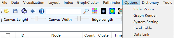
Click on the toolbar ![]() ,or the menu bar “Options” -> “Graph Render”, pop-up graphics rendering settings toolbar or panel as shown below:
,or the menu bar “Options” -> “Graph Render”, pop-up graphics rendering settings toolbar or panel as shown below:

Click on the graphic style panel ![]()
![]()
![]()
![]()
![]()
![]()
![]()
![]()
![]()
![]() ,switch the display style of the node, as shown below.
,switch the display style of the node, as shown below.


Click in the graphics panel ![]() ,the nodes are all of the same size and can be used in various analyses. Click again to indicate that the size of the nodes is inconsistent, and is proportional to the number represented by the node.
,the nodes are all of the same size and can be used in various analyses. Click again to indicate that the size of the nodes is inconsistent, and is proportional to the number represented by the node.
Click in the graphics panel ![]() ,to distinguish between selected and unselected nodes, two colors will be used. You can select a node by clicking on it.
,to distinguish between selected and unselected nodes, two colors will be used. You can select a node by clicking on it.
After selecting some nodes on the left side of the software, click on the envelope icon, as shown in the screenshot below:
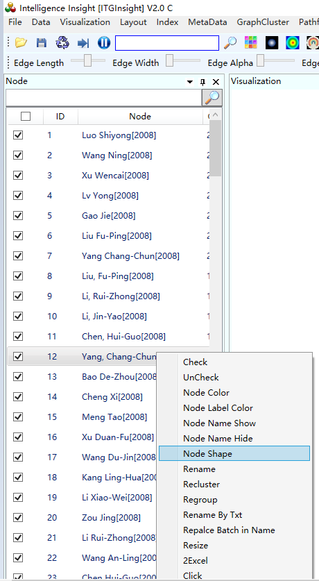
To modify the shape of a node, you can select it and then use the mouse + shift key to select multiple nodes in the graphics area. Once selected, you can modify the shape of the node, as shown below.

To change the color of a node, you can double-click the style option in the style panel, which will open a color dialog box. From there, you can select different colors and the node color in the graphics area will change accordingly.
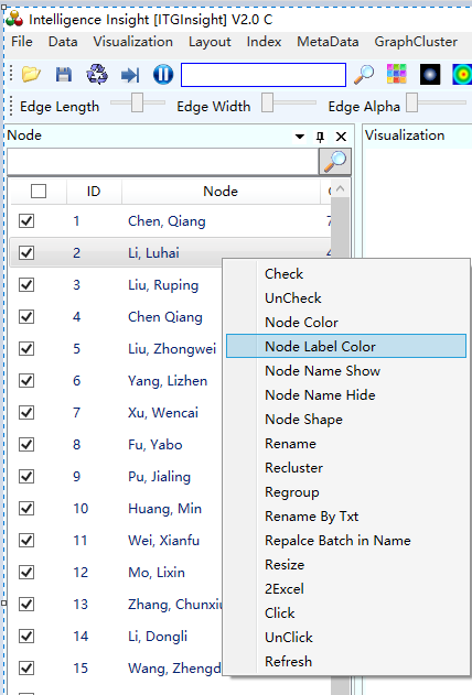
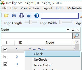
Alternatively, you can also personalize the color of a node from the node content panel on the left side of the main page. First, select one or more nodes using the left mouse button, and then right-click on “color”, as shown below.
If you want to change the color of multiple nodes at once, you can use the mouse + shift key in the graphics area to select them all at the same time.
Click on the toolbar ![]() ,pop up the node coloring options as follows:
,pop up the node coloring options as follows:
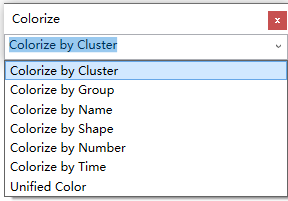
Nodes can be colored based on the relationship strength, node name, node shape, and node size. These coloring options are available when using a single machine for analysis.
Click on the style panel ![]() ,switch node border display or not, double click to change node border color.
,switch node border display or not, double click to change node border color.
Click on the graphic style and click on the style panel. ![]() ,all nodes have the same line width by default, which is suitable for various analyses. However, you can click again to indicate that the node connection widths are inconsistent. In this mode, quantity comparison can be used for co-relationship analysis and co-occurrence relationship analysis. The line width represents the quantity of the relationship. Alternatively, in association analysis, the strength of the representation relationship can be used to indicate the width of the node connection.
,all nodes have the same line width by default, which is suitable for various analyses. However, you can click again to indicate that the node connection widths are inconsistent. In this mode, quantity comparison can be used for co-relationship analysis and co-occurrence relationship analysis. The line width represents the quantity of the relationship. Alternatively, in association analysis, the strength of the representation relationship can be used to indicate the width of the node connection. ![]() Indicates that the two nodes of the connection have an initial end relationship and are used in the analysis of the citation relationship. Click in the graphic style panel
Indicates that the two nodes of the connection have an initial end relationship and are used in the analysis of the citation relationship. Click in the graphic style panel ![]() Indicates the number of connections on the wire, click on the hidden quantity again, and can be used in various relationship analysis.
Indicates the number of connections on the wire, click on the hidden quantity again, and can be used in various relationship analysis. ![]() Indicates that the line is a straight line or a curve. Clicking continuously will toggle between displaying the line and the curve. If a single curve is selected, there will be multiple curve styles available, as shown below.
Indicates that the line is a straight line or a curve. Clicking continuously will toggle between displaying the line and the curve. If a single curve is selected, there will be multiple curve styles available, as shown below.

Click in the graphics panel ![]() ,Indicates whether the color of the connected line owned by the selected node is different from other connections. Default view shows no difference between nodes. After the first click, the display remains the same, but after the second click, differences are displayed. Clicking a third time will display the indirectly connected nodes separately from the selected node.
,Indicates whether the color of the connected line owned by the selected node is different from other connections. Default view shows no difference between nodes. After the first click, the display remains the same, but after the second click, differences are displayed. Clicking a third time will display the indirectly connected nodes separately from the selected node.
To change the color of the connection, double-click the “style” option in the style panel. This will open a color dialog box where you can select a different color. The color of the connection in the graphics area will update accordingly.
If the edge is a uniform single color, double-click ![]() to change the text color of the edge.
to change the text color of the edge.
When the connection color is a gradient color, to modify the color of the edge, you need to first select the edge and then right-click to modify the color of the edge’s text. There are three ways to select the edge: 1) hold down Ctrl and click the left mouse button, 2) hold down Ctrl and drag with the left mouse button to form a subgraph, and 3) right-click on any position away from the node in the visualization area to modify the color of the text for all edges.
The system offers three modes for displaying node annotations: 1. Clicking a node with the mouse will display the annotation of the selected node; 2. The annotation of all nodes can be displayed; 3. All node annotations can be hidden.
By clicking ![]() or
or ![]() switch between the three modes, the default mode is the first mode.
switch between the three modes, the default mode is the first mode.
![]() and
and ![]() the difference is that the font size of the node annotation is scaled according to the number represented by the node, and the effect is as follows.
the difference is that the font size of the node annotation is scaled according to the number represented by the node, and the effect is as follows.
When clicking ![]() , if the node text has time information, the node text switches between displaying the node text information or not.
, if the node text has time information, the node text switches between displaying the node text information or not.
In addition to the default way of displaying node annotations using their names, the system also offers two alternative methods: displaying the node number and displaying the node comments, as shown below.

The node number represents the numerical value associated with the node, while the node name and remarks are displayed as text. Switch by clicking in the graphic style ![]()
![]() panel.
panel.
To change the color of the connection, double-click the “style” option in the style panel. This will open a color dialog box where you can select a different color. The color of the connection in the graphics area will update accordingly.
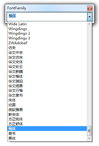
Click ![]() on the toolbar to pop up the node font setting form, as shown below, you can set the font of the node text.
on the toolbar to pop up the node font setting form, as shown below, you can set the font of the node text.
To change the capitalization of node text in the node list area by right-clicking on a selected node, please refer to the following image.

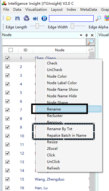
To modify the node content, select one or more nodes by left-clicking on them in the node content panel on the left side of the main page. Then, right-click and choose one of the following options:
“Rename”: This allows you to change the name of the selected node.
“Rename By Txt”: This option allows you to modify the names of multiple nodes at once by matching them to each line in a TXT file.
“Replace Batch In Name”: This option enables you to replace some characters, such as spaces, in the node names in bulk.
These options are shown in the figure below, and can be used to personalize the node names according to your preferences.
Click the style panel ![]() to display the position of the node text in the center of the node or the right side of the node. By clicking on the node annotation multiple times, you can toggle between the three display options: displaying the node name, displaying the node number, and displaying the node comments.
to display the position of the node text in the center of the node or the right side of the node. By clicking on the node annotation multiple times, you can toggle between the three display options: displaying the node name, displaying the node number, and displaying the node comments.
To optimize the display of node labels, right-click on “Node Label Optimize” in the visualization area, as shown in the figure below. This will select an algorithm that automatically adjusts the node label display and hides a portion of the node text.

To resize or change the size of a node, right-click on it in the node content panel and select “Resize/Change Node Size,” as shown in the figure below:

You can specify the node size in a txt file, such as the nodesize.txt file in the example\txt directory. The first column of the file is the node ID, and the second column is the new node size. If the ID of a node in the visualization area matches the ID in the first column of the txt file, the size of that node will be changed accordingly.
To adjust the node size contrast when displaying nodes according to their size, use the Size Variation slider, as shown in the figure below.

To modify the category colors, right-click in the visualization area and select “Cluster Color/Cluster Color”. The category color adjustment panel will appear, as shown in the figure below. Select the corresponding category color to modify, and the modified color will be saved in the file “colors/clustercolors.txt” in the software directory. When using clustering, the category colors will be displayed according to the new settings.


1)Click ![]() on the toolbar, or the menu bar “Options” -> “Slider Zoom”, pop-up slider settings toolbar or panel, as shown below.
on the toolbar, or the menu bar “Options” -> “Slider Zoom”, pop-up slider settings toolbar or panel, as shown below.

2) The following are the available settings for customization: “Canvas Length”, “Canvas Width”, “Side Length”, “Side Width”, “Side Threshold”, “Side Labeling”, “Side Arrow”, “Node Radius”, “Node Border”, “Node Transparency”, “Node Labeling”, “Node Labeling Threshold”, “Node Labeling Angle”, “Node Labeling Transparency”, “Node Remarks”, “Last N Nodes”, “Label Size”, “Thermal Aperture Size, Length, Number, and Ratio”, “Evolution Analysis”, and “Graphic Zoom”.
3.15 Graphics zoom, pan, stretch, rotate
The graphic can be zoomed in or out using the slider setting. The position of the graphic node can be adjusted by dragging it with the mouse, and by holding down the shift key while dragging the mouse, the graphic can be moved. The horizontal stretching of the graphic can be achieved by using the mouse wheel and pressing the left or right arrow keys, while the up and down arrows of the mouse wheel can be used to stretch the graphic vertically.
Through the toolbar ![]()
![]() realize the graphics to rotate clockwise or counterclockwise.
realize the graphics to rotate clockwise or counterclockwise.
Through the toolbar ![]()
![]() to flip the graph up or down or left and right.
to flip the graph up or down or left and right.
The system provides default Chinese and English language options. Click on “Language” in the menu bar to select the language, as shown below:

If you want to operate the software in Japanese, Korean or any other language, please contact the developer and we will provide a version of the software in your preferred language. To set a non-Chinese or non-English language, select “Other” from the language options.
3.17 Change the background color and background border
Click on the toolbar ![]() to bring up the color dialog box and select the color to set the background color of the graphics area. If you want to quickly switch the background color between black and white, click the button on the toolbar
to bring up the color dialog box and select the color to set the background color of the graphics area. If you want to quickly switch the background color between black and white, click the button on the toolbar ![]() . Click on the toolbar
. Click on the toolbar ![]() , the background displays the grid, click again, the background does not display the grid; double click to pop up the color dialog box, select the color, determine the color of the grid.
, the background displays the grid, click again, the background does not display the grid; double click to pop up the color dialog box, select the color, determine the color of the grid.
Enter the name of the node you want to find in the toolbar ![]() , click , the
, click , the ![]() graphic display area will highlight the name of the node being searched.
graphic display area will highlight the name of the node being searched.
The left side of the main page displays information such as the node name, ID, clustering result, and number of connected edges.You can control ![]() the display of power saving or not. To control the display of multiple nodes simultaneously, hold down the shift key, click on the node names on the left side of the screen, and then right-click.
the display of power saving or not. To control the display of multiple nodes simultaneously, hold down the shift key, click on the node names on the left side of the screen, and then right-click.

Right click on the popup menu as follows:
Batch control of node display can be achieved by checking/unchecking the corresponding checkboxes. It should be noted that removing a node will restore its display, and this process cannot replace the layout algorithm.
If you need to delete a node with no connecting lines in the graph, right click ![]() in the graphics area.
in the graphics area.
Additionally, in the graphics area, you can select an area by holding down the Ctrl key and using the mouse, then delete the nodes within or outside this area.Click ![]() and click
and click ![]() separately.
separately.
3.20 Calculate network density, node centrality and main path metrics
(1) To calculate the network density, click on Index/Indicator -> Density/Density in the menu bar, as shown in the figure below.

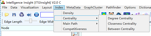
(2) To calculate the point centrality, proximity centrality, and betweenness centrality of nodes in the network graph, click on Index/Indicator -> Centrality/Centrality in the menu bar. The operation is shown below. For the concept and application of relevant centrality, please refer to the academic paper “Research on the Effectiveness of Network Centrality for Journal Citation Evaluation” under the paper folder.
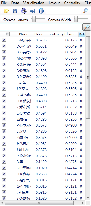
The calculation result will display the node details on the left side of the software, as shown below.
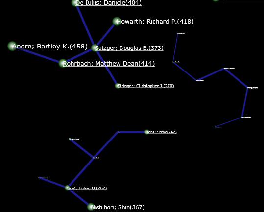
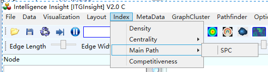
(3)Click on Index/Indicator -> Main Path/Main Path in the menu bar to calculate the SPC values of nodes in the network diagram. The results will be displayed on the left side of the software, as shown in the figure below. For a better understanding of the concept and application of the main path, please refer to the academic paper “Review and Prospect of Patent Citation Network Main Path Method Research_Zhang Xian” under the paper folder. The viewing method for the calculation results is the same as that for centrality.
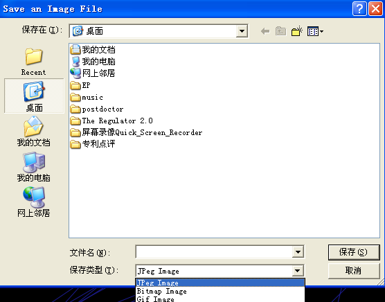
Click on the toolbar ![]() to pop up the graphic file save dialog box, and follow the prompts to save the analyzed image, as shown below.
to pop up the graphic file save dialog box, and follow the prompts to save the analyzed image, as shown below.
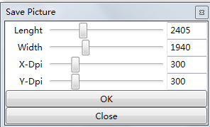
The screenshot’s size and resolution are depicted in the figure above. A higher xdpi and ydpi result in a clearer image but also increase the file size. The default value of 300 is usually sufficient for printing purposes. After taking the screenshot, remember to save the file.
After opening an itgn file, click ![]() directly on the toolbar. The system will generate various statistical data, which are similar to the content of the word report. Additionally, the report list will be added to the first sheet.
directly on the toolbar. The system will generate various statistical data, which are similar to the content of the word report. Additionally, the report list will be added to the first sheet.
You can open a mode file or an itgn file for co-authoring, co-occurrence, association, and citation analysis. After a graph is displayed in the graph area, directly click ![]() on the toolbar, the system can extract node data from the graph and export it to a Microsoft Excel table, which is visualized in the following diagram.
on the toolbar, the system can extract node data from the graph and export it to a Microsoft Excel table, which is visualized in the following diagram.

The system can extract node data from the graph and export it to a Microsoft Excel table, which is visualized in the following diagram.
3.23 Excel report output content settings
By default, the system’s Excel report only provides one-dimensional statistical reports, such as trends and shares. However, if you need more detailed information, you can access the “Options” -> “Excel Table” settings and make additional configurations, as shown below.

The report generation time increases as more output content is selected. Additionally, when analyzing a large itgn file, the data conversion process in version 3.1 may take longer. For instance, when analyzing SCI papers, the maximum number of analysis reports can reach up to 90. In such cases, it is recommended to use Excel for outputting the analysis reports.
ITG Insight provides the automatic write report function of the computer. First open an itgn file, click on the toolbar ![]() , and the smart report dialog box pops up as follows:
, and the smart report dialog box pops up as follows:
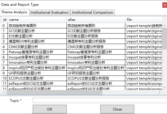
To generate a report, select a suitable template, enter the technical field in the topic/subject section, and click “OK”. The software will automatically generate a comprehensive report, which you can modify as needed based on the prompts.
Please note that the Enterprise Edition of the system provides two default report templates exclusively for top-level users, which are not available to regular users. If you need to customize reports for other data sources or reporting models, ITG Insight offers additional templates, but this may require a technical service fee.
Click on the toolbar ![]() , the system will print the graphics directly on Microsoft Power Point, the effect is as follows:
, the system will print the graphics directly on Microsoft Power Point, the effect is as follows:
This feature requires Microsoft Office 2007 or a newer version to be installed.
3.26 Open save mod graphic file
For each analysis, in order to save the current analysis results, click on the toolbar ![]() , or “File” -> “Save” in the menu bar, save the current analysis results as *.mod files. On the next use, just click on the toolbar
, or “File” -> “Save” in the menu bar, save the current analysis results as *.mod files. On the next use, just click on the toolbar ![]() , or the menu bar “File” -> “Open”, navigate to the *.mod file to open. The content saved in the mod file includes three aspects: 1) node location information, 2) graphic style information (color, threshold, size, length, thickness, etc.), and 3) node content information (node text, remarks, quantity, time, etc.).
, or the menu bar “File” -> “Open”, navigate to the *.mod file to open. The content saved in the mod file includes three aspects: 1) node location information, 2) graphic style information (color, threshold, size, length, thickness, etc.), and 3) node content information (node text, remarks, quantity, time, etc.).
3.27 Open the save layout location information file (reuse of location information)
To ensure consistency in the node positions, it is recommended to save the position information in the mod file for each analysis. This will prevent any changes in the node positions with the same name in the subsequent analyses, click on the toolbar ![]() , or “File” in the menu bar “Save” to save the current analysis result as a *.layout file. On the next use, just click on the toolbar
, or “File” in the menu bar “Save” to save the current analysis result as a *.layout file. On the next use, just click on the toolbar ![]() , or the menu bar “File” -> “Open”, navigate to the *.layout file, you can make the same name node position unchanged.
, or the menu bar “File” -> “Open”, navigate to the *.layout file, you can make the same name node position unchanged.
3.28 Open save graph style information file (reuse of style information)
To save the current adjusted style information, which corresponds to the second type of information, it is recommended to include it in the mod file for each analysis, click on the toolbar ![]() , or the menu bar “File” -> “Save”, save the current analysis result as a *.Graph style file. On the next use, just click on the toolbar
, or the menu bar “File” -> “Save”, save the current analysis result as a *.Graph style file. On the next use, just click on the toolbar ![]() , or the menu bar “File” -> “Open”, navigate to the *.Graph style file to open.
, or the menu bar “File” -> “Open”, navigate to the *.Graph style file to open.
3.29 Visual graphics interact with document data
It is crucial to ensure that each visual graphic corresponds to an original data source. If the data source is saved in Access or Excel, you can interact with the original data through the graphic. To specify the data source of the visual graphic, click the “Data link” or “Data connection” option as shown below:
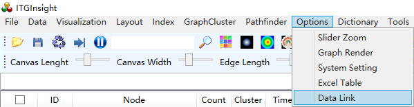

To retrieve the original data through the visual graphic, navigate to the Access or Excel data source used for the visualization, and specify the table to be applied, as well as the filter used in the analysis.
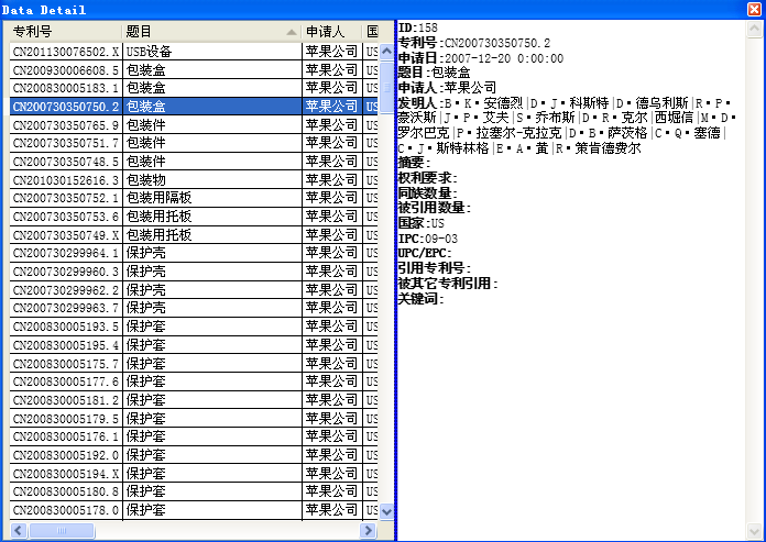
To view the document data corresponding to a visual element, double-click on the node or line in the visual graphic output. By default, only the document data corresponding to the node will pop up. However, if you want to view the document data corresponding to the connection, please note that , click on the toolbar to display the connection data. (This function is limited to Access and Excel data files, and not applicable to data files stored in TXT.)
![]()

To adjust the content displayed in the visualization area, simply move the mouse to the blue line and make necessary changes. For further information about any line in the left table, double-click it and the right side will display additional details, as illustrated below.
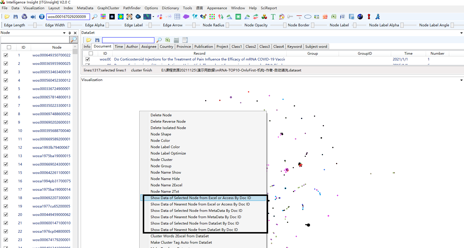
If the graph is a cluster graph obtained through cluster analysis in 6.8, right-click with the mouse button (as shown below) to connect to the original data.
Press to export the coordinates, the coordinate file format is .tsv format.To export coordinates, press the export button and save the file in .tsv format.
To export the legend in the visualization area, right-click on Length/Legend, and export it to PPT where you can make modifications.
3.32 Draw all visual graphics into Word at once
After opening the .itgn file, click on DrawingRobot/Drawing Robot in the toolbar, and the software will automatically draw all graphics in Word. Below is the graphics catalog for the analysis graphics of the SCI paper.
At the same time, users can find mod vector graphics and PNG screenshots of all graphics in the software report template directory, allowing them to edit the mod vector graphics.
The software also offers several shortcut key operations, which are listed in the table below:
| Shortcut operation | |
| Features | hot key |
| Select multiple nodes as subgraphs in a rectangular manner | Press the left mouse button + Ctrl key, move the mouse |
| Select a node connected to a node as a subgraph | Ctrl+Shift key, left mouse click on a node |
| Select edge, modify edge color, modify edge text color: | Ctrl + left click with mouse. |
| Pan the entire graph | Press the left mouse button + Shift to move the mouse |
| Pan subgraph | Press the left mouse button + Shift to move the mouse |
| Orphaned nodes are evenly distributed on the edge of the page | key C or c |
| Graphics optimization start/pause | Enter |
| Translation labels or chronological labels for evolutionary analysis | Press the left mouse button + Alt, move the mouse |
3.34 Saving vector graphics in SVG format
In addition, when saving vector graphics in SVG format, users can customize the image size, font type, and color scheme. This allows users to create high-quality vector graphics that meet their specific needs and preferences.
It’s important to note that the SVG vector graphics feature is only available in version V2.3 or later. If you’re using an earlier version of the software, you may not have access to this feature.
Here are the steps:
Open the MOD file containing the vector graphics you want to save in SVG format.
Click on “Save/保存” in the menu bar.
Select “Svg/矢量图” from the drop-down menu.
Choose a name and location for the SVG file, and click “Save/保存”.
Customize the image size, font type, and color scheme as desired.
Click “OK” to save the changes and generate the SVG file.
Once the SVG file has been saved, it can be opened and edited using any software that supports SVG format, such as web browsers or vector graphics editors.
Please note that some types of vector graphics, such as heatmap, clustering, and density plots, may not be supported in SVG format. If you have any questions or concerns about saving vector graphics

Click ![]() on the toolbar, or “File” -> “Exit” in the menu bar to exit the system safely.
on the toolbar, or “File” -> “Exit” in the menu bar to exit the system safely.
Chapter 4: Cluster Analysis, Thermal Map/Topographic Map/Density Map, World Map, Weather Map, Matrix Map Visualization
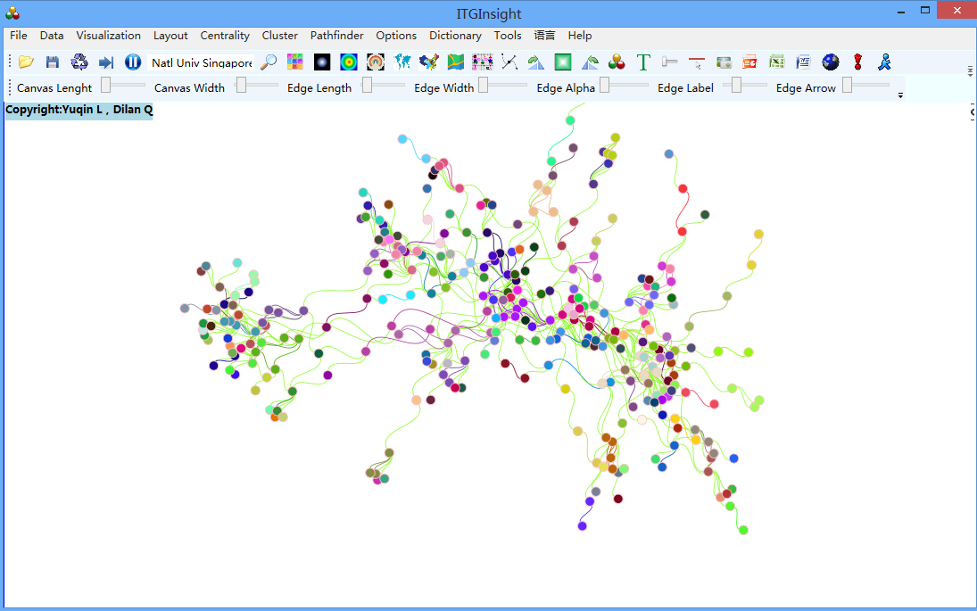
4.1 Network Graph Clustering Analysis
In co-authoring, co-occurrence, coupling, correlation, and citation analysis, clustering the network graph can lead to a clearer representation of the network structure, especially when the number of nodes in the graph is large. The following steps can be taken to cluster the network graph:
1)Click on the menu bar “GraphCluster/Graph Clustering” -> “Vosviewer Algorithm” or “LinLog Algorithm” or “Kmeans(N)” -> “Do/Execute” or “UnDo/Undo” to cluster the network, or cancel the clustering. The first two clusters’ numbers are determined by the algorithm and cannot be adjusted, while the default number of Kmeans (N) clusters is 5, which can be adjusted through the slider panel.

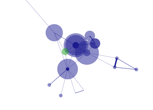
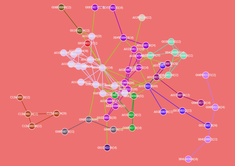
2)View the clustering result in the node content panel on the left side of the main page. Node categories can also be distinguished by the node color in the graphic display area. See below for an example.
3) Click ![]() the button on the toolbar, and the display mode of the network clustering diagram will look like the following figure.
the button on the toolbar, and the display mode of the network clustering diagram will look like the following figure.

- Click
 the button on the toolbar, the display mode of the network cluster diagram is as shown in the figure below.
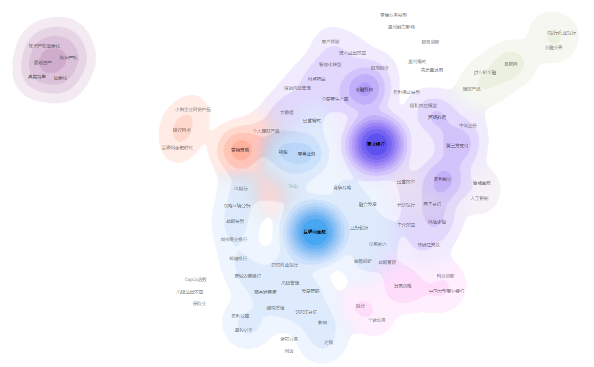
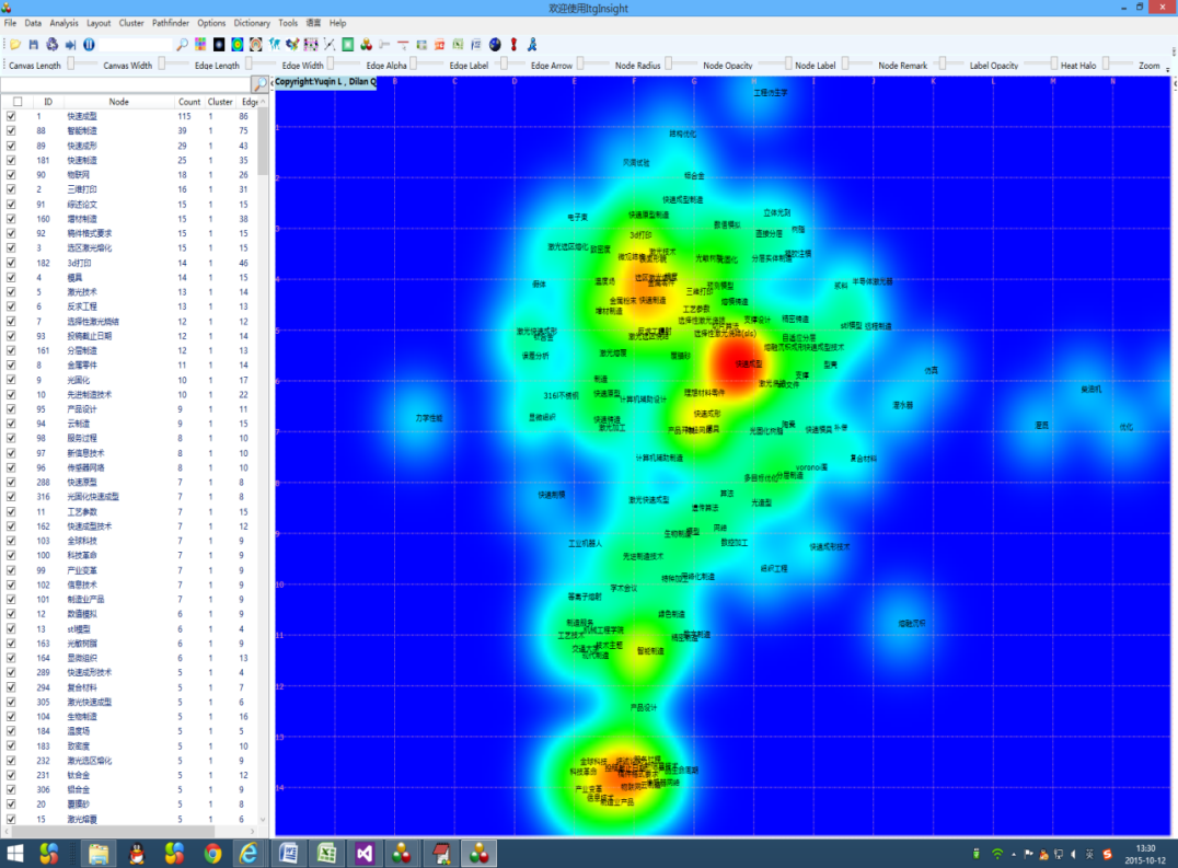
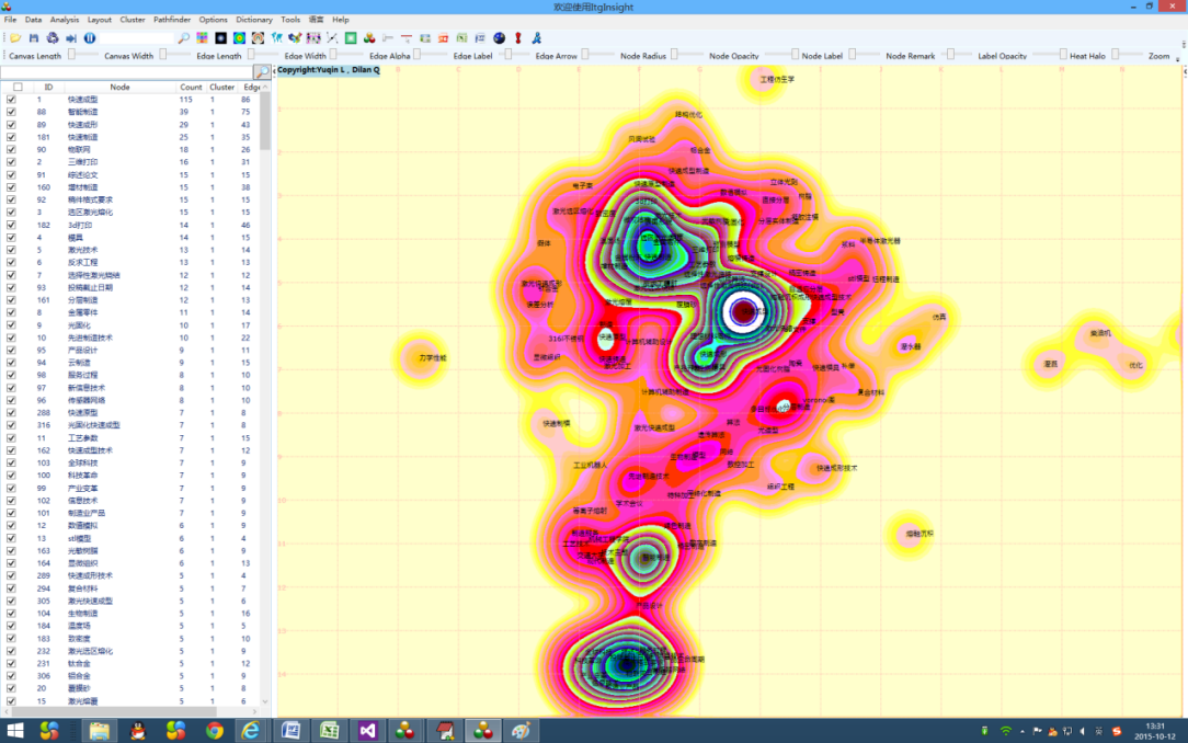
4.2 Thermal map / topographic map / density map visualization
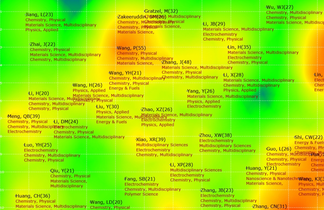
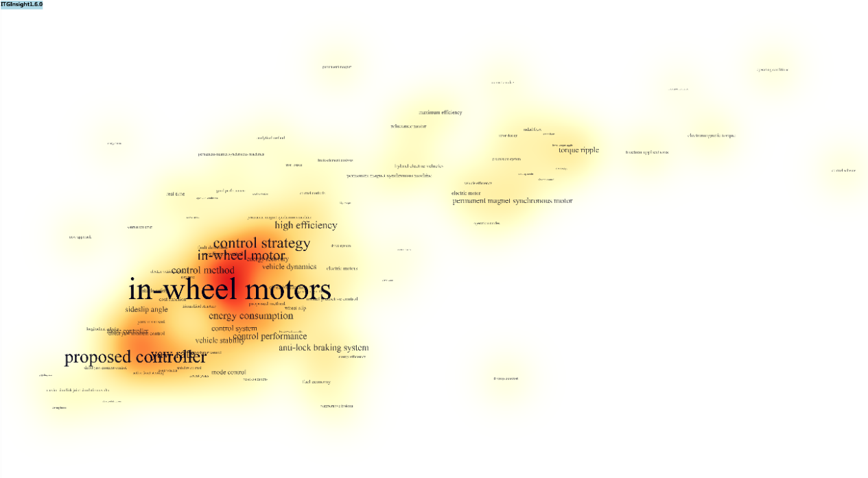
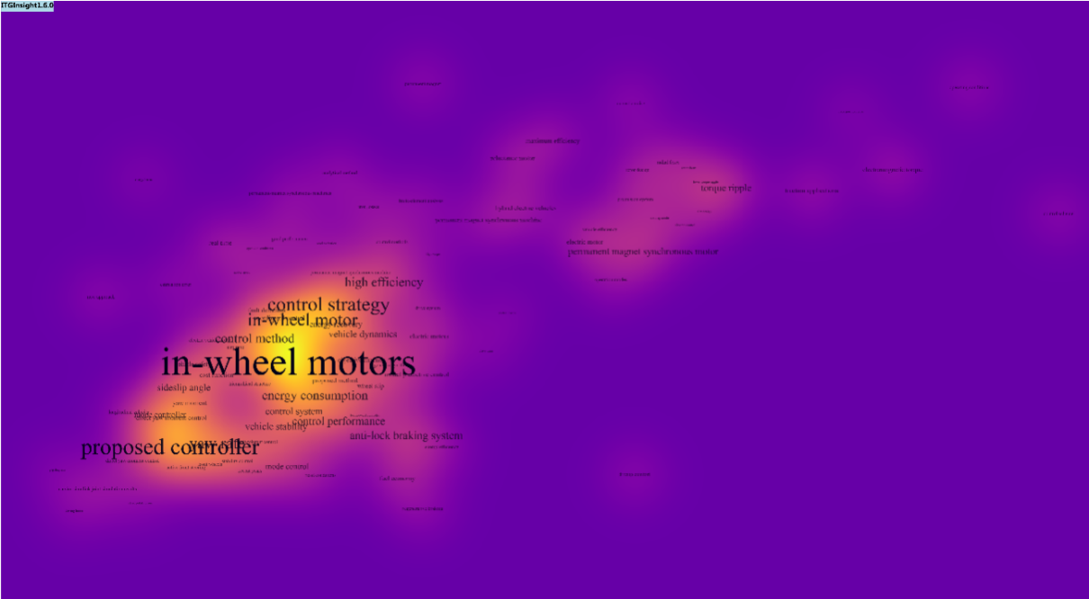
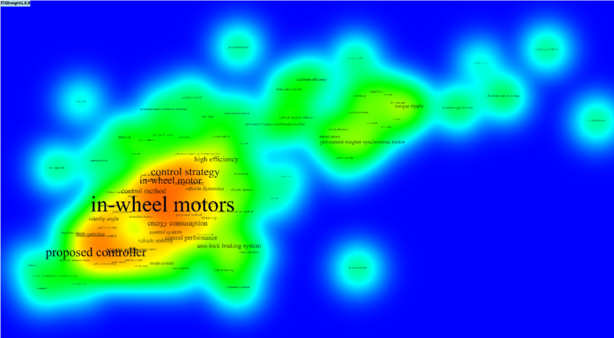
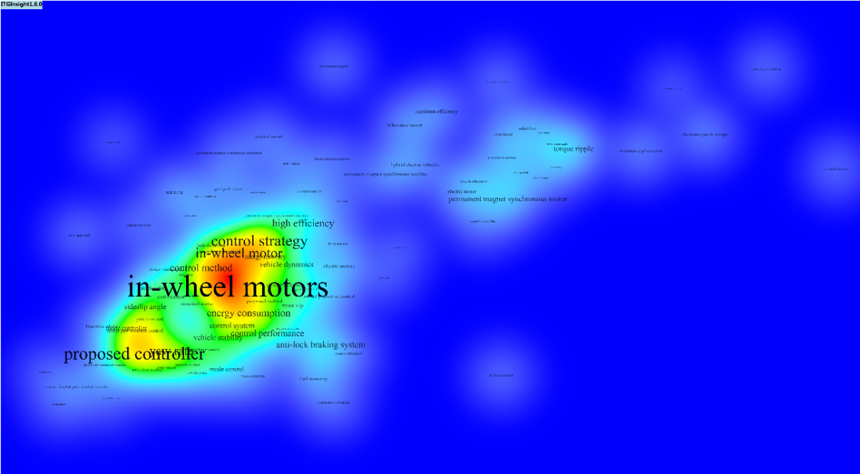
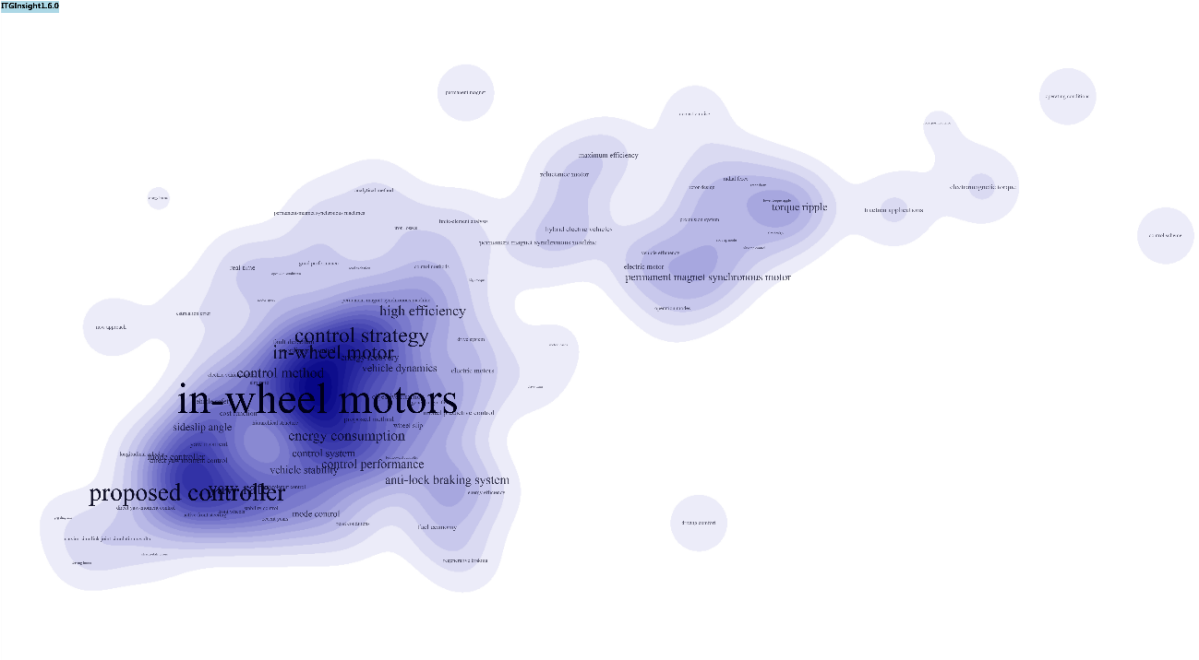
The system’s visualization results are primarily based on network diagrams but also provide heat map, topographic map, and density map visualizations. The heat map simulates the principle of thermal imaging in nature, with the data size represented by four colors: red, yellow, green, and blue. The color block distinguishes the data density. See the figure below for reference.
The specific operation is as follows:

- Click on the menu bar “Layout/Layout” -> “VS Layout or FS Layout.”
- For the network map that has been laid out, click the
 or
or  or
or  button on the menu bar again, and the system prompts the background operation status bar. After the status bar disappears, the graphics area displays the heat map result.
 - Control the display of related content on the heat map/topographic map/density map according to the operation method of 3.9-3.15.
- The V1.6 version adds a theme map similar to VOSViewer. Click the toolbar, as shown below, to access it.
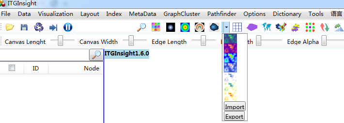
You can customize the style and color of the theme map by importing and exporting functions. Select a color mode after referring to the color format, export it, and observe the color format to make modifications. The following image shows different effects of the same image:

The system provides world map visualization. In the “lalo_world.txt” file in the system installation directory, the latitude and longitude information of major countries in the world is saved. You can add and modify coordinate information in this file, referring to the existing coordinate format. When the node name in the network diagram appears in “lalo_world.txt,” click on the toolbar ![]() and use the world map layout for visual output. The system will determine the coordinates of each node according to their geographic location.
and use the world map layout for visual output. The system will determine the coordinates of each node according to their geographic location.
The system offers China map visualization, where the geographic coordinates of some provinces and cities in China are saved in the “lalo_china.txt” file in the system installation directory. Users can add and modify the latitude and longitude information in the file, following the existing coordinate format. When a node name appears in the network diagram and matches a location in “lalo_china.txt”, users can click on the toolbar ![]() to output a map of China with each node’s coordinates determined by its geographic location.
to output a map of China with each node’s coordinates determined by its geographic location.
Note: For accurate and detailed mapping, users should use more accurate Json data and ensure map correlation. The use of map visualization results must comply with relevant national laws and regulations.
4.5 Matrix Chart Visualization
To convert a network diagram into a matrix diagram, users can click on the toolb ![]() ar to output the nodes of the network diagram as rows or columns of a matrix, the connecting lines of the network diagram as nodes of the intersection of the rows and columns of the matrix, and the graph as a matrix form. Users can click on the row name with the mouse to switch it to a column, and vice versa. Users can also adjust the node text size and color using the same operations as in the network diagram.
ar to output the nodes of the network diagram as rows or columns of a matrix, the connecting lines of the network diagram as nodes of the intersection of the rows and columns of the matrix, and the graph as a matrix form. Users can click on the row name with the mouse to switch it to a column, and vice versa. Users can also adjust the node text size and color using the same operations as in the network diagram.
Note: The condition for converting a network diagram into a matrix diagram is that the nodes in the network diagram are divided into two colors, namely the selected state and the non-selected state. Users can select several nodes on the left side of the software, right-click and click the matrix button to apply the matrix effect.

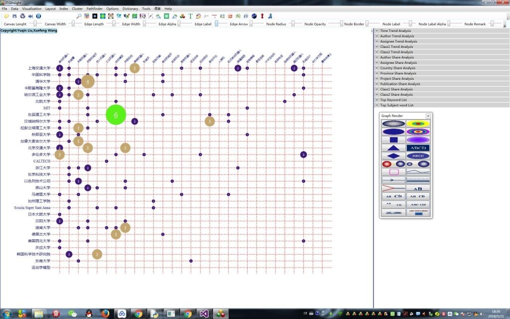
5.1 Use filters to switch analysis objects
ITG Insight is capable of analyzing patents, papers, and reports in both Chinese and English, and offers filters to switch between these analysis objects. The system comes with pre-designed filters for commonly analyzed SCI, CNKI, Derwent, and ItgMining data. The figure below shows an example of a filter that is used to analyze SCI data downloaded from Web of Science.

The <ID><Abstract>….<Title> structure under the <FileMap></FileMap> node is used to set the corresponding field names in the access (Excel or txt) database, as long as the patents, reports, and papers corresponding to these nodes are set. This allows for the corresponding data to be stored in the database.
The <Source> field represents the data source, which can be WOS, CNKI, ITGMining, or any other default source.
The <ID> field corresponds to the unique standard field and must exist; otherwise, an error will occur.
Other fields include <Abstract> for the summary field,
<Authors> for the author field,
<Affiliation> for the corresponding affiliation field,
<Class1-4> for the category fields,
<Keyword> for the keyword field (which can correspond to multiple fields),
<Countries> for the region field,
<Publication> for the journal field,
<Description> for the text field,
<Reference> for the reference ID,
<ReferencedBy> for the cited document ID,
<Time> for the time field,
<Title> for the title field.
In addition, there are optional fields that are only relevant to some filters and are mainly used to convert literature into reference format.
These fields include <Cities> for cities,
<PublicationTime> for publication time,
<PublicationType> for publication type,
<PublicationArea> for publishing area,
<Publisher> for publisher,
<Volume> for volume,
<Period> for period,
<PageStart> for start page,
<PageEnd> for end page.
If the corresponding field does not exist, no content will be filled in the corresponding part, such as the <Description> node in this example.
5.2 Analysis threshold, parameter setting
The contents within the <System></System> node in sysset.xml are used to configure parameters related to the system or analysis.
<SoftName> is utilized to modify the interface display name after the software is launched;
<SoftCopyRight> is used to define the copyright information located in the upper left corner of the page after the software is launched;
<VSMwordMax> is used to specify the maximum number of words for semantic calculation. The higher the number, the greater the hardware requirements and longer the calculation time;
<StopWordFile> is used to set the path of the stop word file, which is set as the default value “stopwords.txt”;
<ThesaurusFile> is used to set the path of the subject file, which is set as the default value “thesaurus.txt”;
<DataFile> is used to set the path of the Access data file;
<CoThreshold> is used to determine the threshold for co-existing analysis. If the threshold is exceeded, the co-calculation calculation is performed on the graph and displayed as “wired”;
<CoreThreshold> is used to set the threshold associated with correlation analysis and association analysis. If the value is exceeded, the correlation calculation is considered, and the graph is represented as having a “connection”.
<OnlyEdgeCoauthor> is used to specify whether to output only nodes with a co-author relationship when outputting the author’s merging graphics;
<OnlyEdgeCoassignee> is used to specify whether to output only nodes with a co-assignee relationship when the output mechanism is merging the graphics;
<OnlyEdgeCocountry> is used to specify whether to output only nodes with a co-country relationship when merging graphics in the output area;
<OnlyEdgeCoclass1> is used to specify whether to output only nodes with co-occurrence relationship when outputting the category 1 co-occurrence graph;
<OnlyEdgeCoclass2> is used to specify whether to output only nodes with co-occurrence relationship when outputting the category 2 co-occurrence graph;
<OnlyEdgeCoword> is used to specify whether to output only nodes with co-occurrence relationship when outputting keyword co-occurrence graphics;
<OnlyEdgeDocumentReference> is used to specify whether to output only nodes with the citation relationship when exporting the document citation graph;
<OnlyEdgeAuthorReference> is used to specify whether to output only nodes with the citation relationship when outputting the author citation of the co-occurrence graph;
<OnlyEdgeAssigneeReference> is used to specify whether only nodes with citation relationship should be outputted when citing the graph;
<OnlyEdgePublicationReference> is used to specify whether only nodes with citation relationship should be outputted when exporting journal citation graphics;
<OnlyEdgeDocumentCoReference> is used to specify whether only nodes with coupling relationship should be outputted when outputting document coupling graphics;
<OnlyEdgeAuthorCoReference> is used to specify whether only nodes with coupling relationship should be outputted when outputting author coupling graphics;
<OnlyEdgeAssigneeCoReference> is used to specify whether only nodes with coupling relationship should be outputted when the output mechanism is coupled to the graph;
<OnlyEdgePublicationCoReference> is used to specify whether only nodes with coupling relationship should be outputted when outputting the publication coupling graph;
<OnlyEdgeCountryCoReference> is used to specify whether only nodes with coupling relationship should be outputted when coupling graphics in the output country;
<PFNET> is used to set whether the network map should be compressed by the computer.
You can also set these parameters by going to “Options” -> “System Setting”, as shown below, or by specifying the settings of the above parameters when performing data conversion.
If there are irrelevant words in the analyzed text related to the keywords, such as “of,” “in,” “on,” “land,” “de,” and so on, you can eliminate these keywords by configuring stop words (most of which have been removed by default by the system). The stop word setting is located in the dic/stopwords.txt file in the system installation directory, with each stop word on a separate line. After setting up the stop words, restart the program and the vocabulary will be updated accordingly. You can specify the path of the stop word file in “Options” -> “System Setting” -> “Dictionary,” as shown below. Alternatively, you can specify the stop word file path when converting data.

Additionally, you can add or remove stop words in “Dictionary/Dictionary” -> “Stop Words/Stop Words,” as shown below.

Note that stop words are not case-sensitive.
In order to split the words according to user-specified words in the analysis of digest words, you can use thesaurus-based word splitting, also known as keyword segmentation. The setting of the keywords is in the dic/thesaurus.txt file in the system installation directory, where the format is as follows:
Word A1|Word A2|Word A3|Word A4|Word A5|Word A6|Word A7|Word A8 – this means that word A1 is replaced by words A2-A8, and|Word B1|Word B2|Word B3 – this means that words B1, B2, and B3 are meaningless words (similar to stop words) and are not included in the statistical range.
After setting up and restarting the program, the thesaurus will take effect and will also play a role in the analysis of keywords. You can specify the path to the thesaurus file via Options->System Setting->Dictionary. You can also add or delete keywords in “Dictionary” -> “Thesaurus”. The method for doing this is the same as for stop words. The use of subject terms can be set to “Apply subject words”, “Use only keywords”, and “Use only words” to determine how the keywords are used. Among these methods, using only keywords is the recommended usage scheme of the software, as it multiplies the amount of data processed and the keywords have more practical meaning. Thesaurus is not case-sensitive.
To standardize the inaccuracies in statistical results caused by differences in writing formats for personal names, the software provides a name dictionary file for correcting name variations. This file, named persondic.txt, is located in the software directory dic/. Modifications to the file are similar to those for subject terms and follow the format:
Person name A1|Person name A2|Person name A3 – meaning replace Person name A2-A3 with Person name A1
|Name B1|Person name B2|Person name B3 – meaning the names B1, B2, B3 are meaningless and not in the statistical range.
By default, the name dictionary is not case sensitive. To differentiate between uppercase and lowercase, add “1” to the first line of the dictionary, and add “0” to indicate case insensitivity.
5.6 Company dictionary setting
To standardize the writing format of organizational names, as well as modifications and mergers, the system provides an institutional dictionary file for correcting organizational names. This file can be found in the software directory dic/corporationdic.txt. The modifications to the file are consistent with those made to the keyword and name dictionaries, and follow a similar formatting pattern:
Organization A1|Agency A2|Agency A3 – this means that mechanism A2-A3 will be replaced with mechanism A1
|Institution B1|Institution B2|Institution B3 – this means that institutions B1, B2, and B3 are meaningless and not in the statistical range.
By default, the company dictionaries are not case sensitive. If you want to distinguish between uppercase and lowercase letters, add “1” to the first line of the dictionary. Adding “0” indicates that case sensitivity is not required.
5.7 Country name dictionary setting
To standardize the statistical results of country names, including name format, modification, and mergers, the system provides a national dictionary file for revising place names. This file is located in the software directory dic/countrydic.txt. The format of the file is consistent with that of the subject words, person names, and institutional dictionaries. For example:
Place name A1|Place name A2|Place name A3 – meaning that the place name A2-A3 is replaced by the place name A1
|Place name B1|Place name B2|Place name B3 – meaning that the place names B1, B2, and B3 are meaningless and not included in the statistical range
By default, the country dictionary is not case-sensitive. To distinguish between uppercase and lowercase, add “1” to the first line of the dictionary. Add “0” to indicate case insensitivity, and add “2” to indicate capitalization.
5.8 Provincial dictionary setting
In order to standardize inaccurate statistical results caused by differences in the writing format of province names, modifications to the province name, mergers and acquisitions, etc., the system provides a provincial dictionary file for the revision of place names. This file can be found in the software directory dic/province-chinese.txt. The modification of the file is consistent with the keyword and name dictionaries. The formatting is similar, as follows:
Place name A1|Place name A2|Place name A3, meaning that the place name A1 replaces the place name A2-A3.
|Place name B1|Place name B2|Place name B3, meaning that the place names B1, B2, B3 are meaningless and are not within the statistical range. By default, the gazetteer is not case-sensitive. If you want to distinguish between upper and lower case, add “1” to the first line of the dictionary. Adding “0” indicates case insensitivity, and adding “2” indicates capitalization.
5.9 Dictionary content case sensitivity setting
In order to standardize the names of persons, organizations, and places in the text, the system allows for case sensitivity settings in the corresponding dictionary files. If the first character in the dictionary is a single number “1”, then the case spelling is strictly distinguished during data processing. Otherwise, the case is not case-sensitive. For place names, the first character is “2”, indicating that the first letter of the place name should be capitalized.
5.10 Apply regular expressions in dictionaries for advanced filtering and replacement
Regular expressions can also be applied in dictionaries to perform advanced data filtering and replacement. For instance, when processing CNKI papers, institutional names may not be standardized and may include postal codes, provinces, and cities as part of the institution name. In such cases, regular expressions can be used to filter out unwanted information and ensure that the institutional name is properly recorded. For example, in the paper “Research on the Influence of Organic Compound Warm Mix Agent on Asphalt Performance”, the institutional information can be modified using regular expressions.
![]()
This information is not exhaustive prior to data cleaning, which can lead to inaccurate data analysis. There are two processing methods:1)If abnormal data is discovered after data cleaning or analysis, use a dictionary to replace or delete the data point one by one, and perform data cleaning or analysis again.2)Before cleaning or analyzing the data, use regular expressions in the institutional dictionary to process it. The institutional dictionary example is shown in the above figure. 
The line starting with “r” in the figure indicates that this line is a regular expression replacement. The basic format is “r|new character after replacement|regular expression finds the character that needs to be replaced”. The new character after the replacement is “”, which means the replacement becomes a deletion.
For example, “r||[0-9]{6}” means to delete the 6-digit zip code. “r||\s\S{3}$” and “r||\s\S{2}$” respectively indicate that the name of the organization with lengths of 3 and 2 characters is deleted. Regular expressions can be used for advanced filtering, deletion, and replacement, but it requires some knowledge of the relevant rules.
5.11 How to set the dictionary when using the software for the first time
When using the software for the first time, start the software and click on the “Initialize Dictionary” button to set up the dictionary. After the initialization process is complete, close the software and then restart it to ensure that the dictionary settings are applied.

ITGInsight provides data cleaning capabilities that allow users to clean their data and generate a dictionary, which can be used for data analysis and visualization without changing the original data.
6.1 Select the data source to be washed
To select the data source for cleaning, users can click on the toolbar “Data” -> “Cleaning” to enter the data cleaning page, as shown below.

They can then select the content to be cleaned, with the operation being consistent with the process described in section 3.1 on data format conversion. While users can choose to use a dictionary at this step, it is not recommended.
After cleaning, the basic information of the data is displayed under the “Information/Info” tab, as shown below.

This page shows the number of records included, along with the number of records recorded for each data category such as author information, institutions, countries, provinces, publications, categories 1, categories 2, keywords, and abstract words. The purpose of displaying this information is to provide a quick overview of the distribution of data across different categories, which can help in understanding the dataset and its characteristics. The difference between these categories lies in the type of information they represent, such as author information including the name and affiliation of the author, institutions representing the organization where the research was conducted, countries and provinces indicating the geographic location, publications indicating the name of the publication where the research was published, and so on.
6.3 Data manual grouping to achieve data cleaning
Under the label of person name, organization, country, province, category, keyword, abstract word, etc., select the record to be cleaned by using the left mouse button + shift, then right-click on “Update Group Menu” to bring up the modify group window, as shown below.

In this window, you can enter the group name.
6.4 Automatic data grouping for data cleaning
Under the labels such as author, organization, country, province, category, keyword, and abstract word, select the records to be cleaned by using the left mouse button + shift, and then right-click on “Update Group Auto”. The automatic grouping window will pop up, as shown below.

Stemming is a process that performs part-of-speech restoration of English data. The similarity function combines data based on their similarity.
If the tag is for a person’s name, the automatic grouping dialog box that pops up will be slightly different, as shown below:

This window provides options for distinguishing whether the author is the same author or a different author. The similarity of the author’s name, institution, country, etc., is used to identify the same name and assign them the same value.
After clicking Close, the system will automatically calculate the similarity of the records. The calculated results will be displayed as shown above.

For example, based on the GroupID, records 381 and 298 are grouped together. The GroupID is the same and the numbers in the brackets represent the similarity. The grouped data is stored as a dictionary, which is considered a record and used as a user dictionary in subsequent analysis. If you believe that the computer grouping is incorrect, you can right-click to select “ungroup” and the group will be restored to its original state.
When performing data analysis, grouped records can be uniformly replaced by new ones. To save a record as a dictionary, simply select it by holding down the left mouse button and pressing shift. Then, right-click to bring up the context menu and select “Check”. Finally, click the button ![]() on the toolbar to output the result as a dictionary in TXT format. Alternatively, you can also save the record as an Excel file and use the toolbar
on the toolbar to output the result as a dictionary in TXT format. Alternatively, you can also save the record as an Excel file and use the toolbar ![]() button to save it as a dictionary.
button to save it as a dictionary.
6.6 Use the dictionary to clean the data again, data analysis, automatic grouping
The dictionary that was saved can be reused for future data cleaning and analysis by storing it in the corresponding directory.
To use the dictionary for grouping, simply follow the steps shown in the screenshot below. By reusing the dictionary, you can avoid duplicating your work.

Grouping words with a dictionary may prompt the user whether to allow a record to be assigned to multiple groups, as shown in the screenshot below.


After cleaning the data, click on the “Save” button on the toolbar to save the result. You can then open the saved file using the “Open” button on the toolbar the next time you use it, as shown in the screenshot below.

The dataset format is the default saving format, which is suitable for cases where the amount of data does not exceed 30,000 records.
The bigdataset format is an optional saving format that removes reference information during the saving process. This format is suitable for cases where the amount of data exceeds 30,000 records.
Due to limitations in the operating system, the size of the data that can be saved is restricted, and the citation information may be too large to be saved. Therefore, during the data cleaning phase, if you don’t require the citation information for analysis, it is recommended to save the data in the bigdataset format.
6.8 Combined analysis (cross-dimensional, cross-level co-occurrence matrix, citation matrix)
To select data in three dimensions of time, author, organization, country, province, category, keyword, and abstract word, check the desired data and right-click to bring up the Combinatory Analysis option, as shown below.

A dialog box will pop up for combined analysis. Here, you can select the row, column, and statistical criteria, as well as the type of analysis to be performed, as shown below:
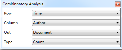
The figure above shows the number of documents after statistical analysis of the intersection of time and author dimensions.
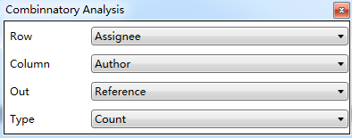
The figure above shows the number of references after statistical analysis of the intersection of author and agency dimensions. This represents the number of documents cited by an author.

The figure above shows a list of references after statistical analysis of the intersection of author and agency dimensions. This list contains the IDs of the documents cited by an author.
After selecting the desired options, close the dialog box, and the system will call Excel to output the statistical matrix, as shown below:


The figure above shows the number of documents after statistical analysis of the intersection of time and author dimensions. Visual graphics can be directly output to the software’s graphics area.
6.9 Grouping statistics (after data cleaning, statistics shall be made according to new groups)
Combination analysis involves performing two-dimensional and three-dimensional statistical analysis on data. When data is grouped and one-dimensional statistics are required, check the desired options to be counted, and then click on “Group Statistics/Group Stat” on the menu bar or use the right mouse button to initiate one-dimensional grouping statistics, as shown in the following figure:
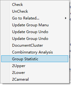
Both group statistics and combination analysis are calculated based on new groups.
To initiate clustering, right-click on the data cleaning interface and select “Cluster/Cluster,” as shown below:

Cluster is used for clustering objects, with documents being the default. The field used for clustering is typically the keyword field, but other fields can be selected as well. The number of keywords used to calculate the document relationship is also customizable. Note that the larger the data, the longer the clustering time.The output content can be a network visualization or a density map, with the color of the network node being determined according to the selected field (e.g., organization or country of the document). By default, the color is distinguished. Note that regardless of the selected field, it must be checked for the clustering to work. If a field is left unchecked, the corresponding documents will not be clustered.
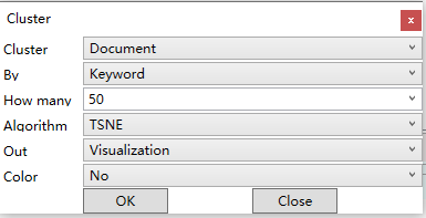
Once the clustering calculation is completed, the resulting network diagram will be displayed in the main form, as shown below:
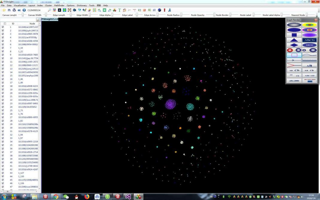
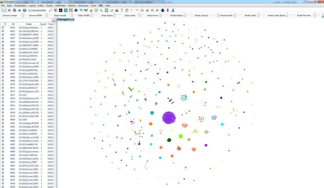

Further label the clustering results, click the right mouse button, as shown below:
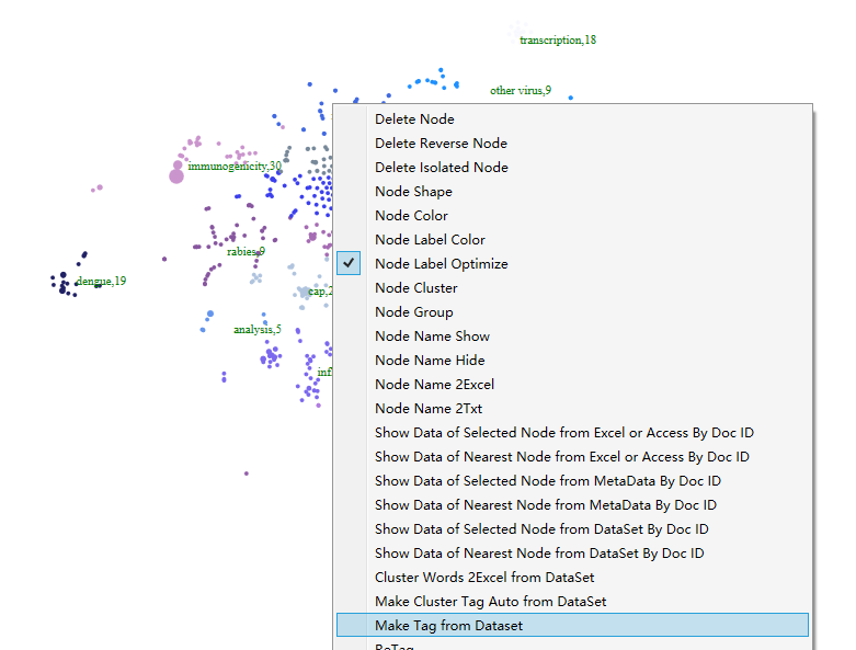
Pop up the input label box: as shown below:

You can manually enter labels for each cluster or category. Additionally, if the data cleaning interface has the dataset corresponding to the clustering map open, the software will suggest category label content. The color of the tags can be changed using the “Tag Color” option from the right-click pop-up menu, and the size of the tags can be adjusted using the tag slider. The resulting clustered map can be seen below.

However, manually labeling each cluster can be time-consuming. To simplify the process, you can use the “Make Cluster Tag Auto from Dataset” function available from the right-click pop-up menu.
In the data list, select data in any dimension, and right-click to navigate to the corresponding data, as shown in the figure below. For instance, if you select any author and click “go to related publication”, you will be directed to the journals corresponding to the papers published by these authors, and so on. You can navigate to any dimension data.
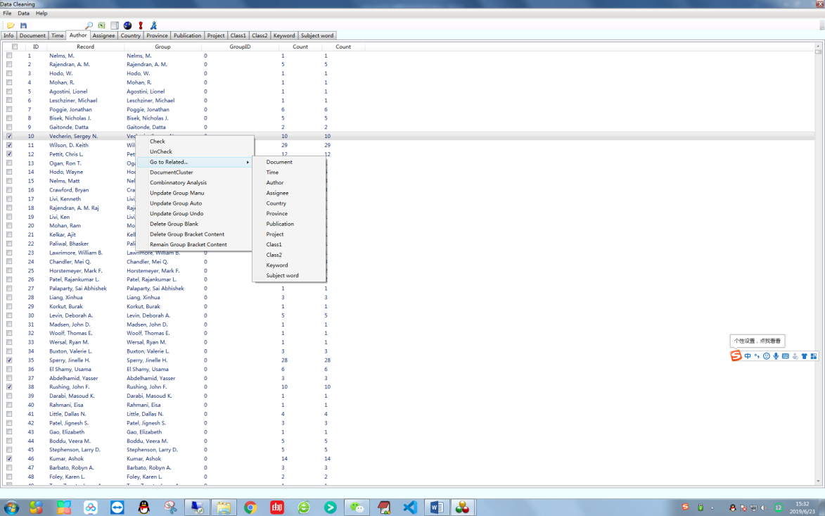
6.12 Convert Dataset to Excel or TXT
Right-click on “Document” in the dataset page, and select “Document to Excel” or “Document to Txt” to transfer the dataset to Excel or Txt files, as shown in the following figure.

Since V2.2, the Dataset page after data cleaning provides visualizations similar to the Data Analysis page, as shown in the screenshot below. To visualize the data, you need to check the corresponding field information to display the results. Note that the visualizations here are based on the cleaned data and do not involve dictionary operations.
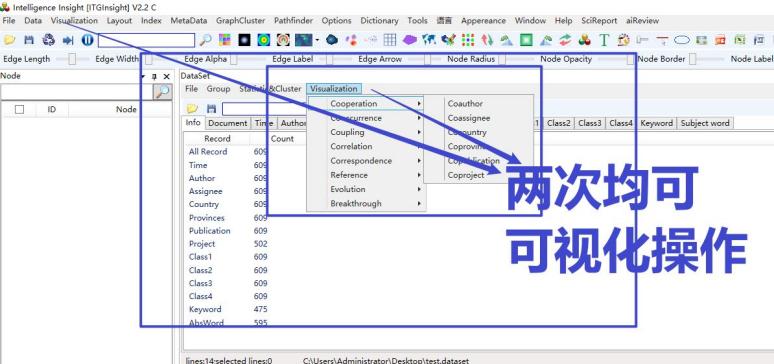
6.14 Convert Dataset to Itgn File
After V2.2, on the dataset page after data cleaning, click the “2ITGN” button on the menu bar to convert the dataset into an ITGN file. The ITGN file generated here is essentially the same as the ITGN file generated from data analysis. It stores the statistics and visualization results of various dimensions, as shown in the following figure. Before conversion, the information to be analyzed must be checked on the Dataset page. Otherwise, there will be no corresponding results in ITGN, and no corresponding dimension statistics and visualization content will be generated.


Chapter 7: Auxiliary Software Tools
7.1 INPADOC family patent visualization analysis tool
Click on “Tools/Tools” -> “ItgFamily/INPADOC Family Analysis” to open the World Patent Family Real-Time Update and Analysis System, ItgFamily, as shown below:
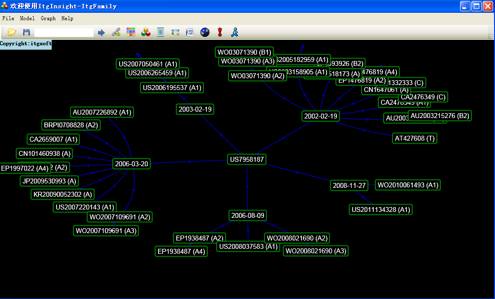
The ItgFamily World Patent Family Real-Time Update and Analysis System is a powerful tool that supports enterprise patent strategy decision-making. The system enables worldwide data collection and tree representation of patents. Its unique feature is the ability to update family applications in different countries at different times and arrange family patents chronologically in a tree structure. The system does not limit the number of patents displayed on the screen. User interaction is performed through mouse double-click and drag, and the analysis graphics are simple, beautiful, and clearly structured. To learn more about the tool, please refer to the corresponding help file, itgfamily help.pdf.
7.2 US Patent Citation Visualization Analysis Tool
Clicking on “Tools / Tools” -> “ItgReference / US Authorized Patent Citation Analysis” retrieves the ItgReference US Patent Citation Validation and Analysis System, as shown below:
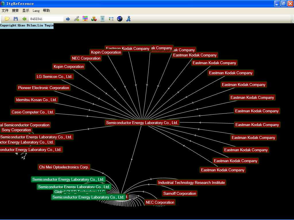
The ItgReference system is a support tool for enterprise patent strategy decision-making. It allows users to collect and analyze citation information from US patents, both in the front and the back. The system displays the citation information in a tree structure and there is no limit to the level of patent citations or the number of patents displayed on the screen. The system is user-friendly, using mouse double-click and drag for interaction. The analysis graphics are visually appealing, and the structure is easy to understand. The system is comparable to Aureka’s patent citation map. The corresponding help file, itgreference help.pdf, is available for reference.
7.3 US Patent Claim Analysis Tool
Click on “Tools” -> “ItgClaims / US Patent Claim Analysis” to access the US Patent Claims System ItgClaims, as shown below:

The ItgClaims US Patent Claims Resolution System, as a subsystem of the general science text visualization mining system ITGInsight, mainly implements the online search, extraction, structural analysis, and visualization of independent claims and dependent claims in US single patent claims. Its biggest feature is the automatic generation of the claim tree, which is displayed in a visual form. There is no limit to the number of claims displayed on the screen. The system uses mouse double-click and drag to perform user interaction, and the analytical graphics are simple, beautiful, and have a clear structure. You can view the corresponding help file itgclaims help.pdf to learn how to use the tool.
Chapter 8: Custom Structured Data Visualization
The ITGInsight system supports visualization of four types of custom format data: .ima, .imb, .imc, and Excel formats.
The first type is the ima format data, which can be found in the software installation directory, for example, in the directory “example\ima”. The format of the data is as follows:
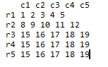
The ima format data is the simplest matrix data, where the data is separated by a single space. The ima format data is only used for data presentation, and it is convenient for users to understand the differences between different layout algorithms. Generally, it is not applied in actual analysis projects.
The second type is the imb format data, which can define nodes and connections for simple visual display. The format of the imb file can be found in the installation directory example\imb file, and is as follows:
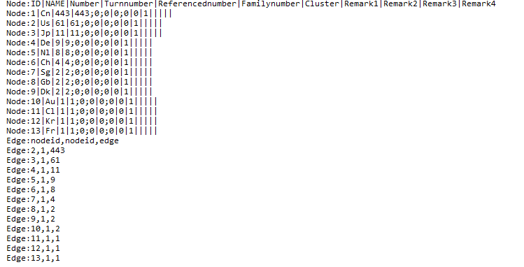
imb format data can define nodes and connections for simple visual display.
Node:ID|NAME|Number|Turnnumber|Referencednumber|Familynumber|Cluster|Remark1|Remark2|Remark3|Remark4
Used to define nodes, where the ID is a node identifier, which is distinguished by 1, 2, 3… and cannot be repeated.;
Name is the node name and will be displayed in the visual graph;
Number is the number of nodes represented;
TurnNumber is the first, second, and third author numbers represented by the node, and the sum must be equal to Number;
Referencenumber is the number of citations and prints of the node, both numbers can be 0.;
FamilyNumber is the number of the same family of the node, a number, can be 0;
Cluster is the category to which the node belongs. The category is numbered 1, 2, 3… or both;
Remark1, Remark2, Remark3, Remar4 are the comment text of the node, up to 4, can be empty.
Edge:nodeid,nodeid,edge
Used to define the connection, nodeid is the number of the starting and ending node, which must be defined in the node definition.;
Edge is the number of lines marked.
The third category is the imc format data files, which are the most flexible and powerful data format, as follows:

Node:NAME|Number|Turnnumber|Referencednumber|Familynumber|Cluster|Remark1|Remark2|Remark3|Remark4|color|shape
Used to define nodes, not the imb format is different, imc format only needs to define the node name, no need to define the node number, but the node name is different.
Color is the node color;
Shape is a node shape, only tender 1 or 0, corresponding to the circle and rectangle.
Edge: nodename|nodename|edge|label|color
Used to define the connection, nodename is the name of the connection start and end point;
Edge is the number of connections;
Label is the text label of the line;
Color is the color of the connection.
8.4 imd format data
The fourth category, which consists of imd format data files, offers even more flexibility. Consider the following example:
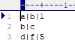
We have a network graph with five nodes, labeled a, b, c, d, and f, and two directed edges: one from a to b with weight 1, and another from d to f with weight 5. The imc and imd formats are suitable for representing network data with single orientation, such as patents transfer transformations, but they can also be used for bidirectional data. For instance, we can add the entry “f|d|3” to represent an edge from f to d with weight 3, and an edge from d to f with weight 5, forming a bidirectional graph.
8.5 Excel format data (universal format)
The fourth category includes data files in Excel format, which can be found in the installation directory under the path “example\excel”. The format of these files is as follows: 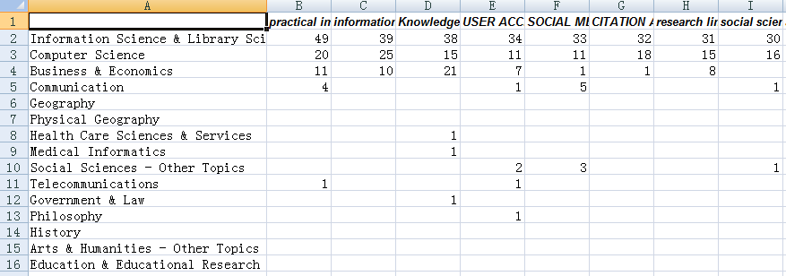
Or as follows:
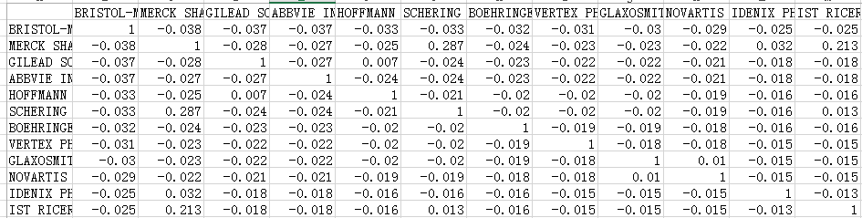
Once the user opens an Excel format file, the system will prompt the user to indicate whether the data to be opened is a frequency matrix, a similarity matrix, or a Pearson matrix. The user can also specify whether to perform matrix operations to obtain the co-occurrence matrix, the correlation matrix, or the corresponding matrix, as shown in the figure. 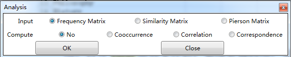
If the user selects the Similarity Matrix, the Pierson Matrix/Pearson Matrix options, the system will not perform any calculation on the matrix by default. Instead, the system will directly convert the matrix into a network diagram.
If the user selects the Frequency Matrix/Frequency Matrix option, no calculation will be performed. If the row and column names of the frequency matrix are exactly the same, the output network graph will be a 1-mode network graph. Otherwise, it will be a 2-mode network graph.
If the user selects any of the remaining three options (i.e., Similarity Matrix, Pierson Matrix/Pearson Matrix, and Co-occurrence Matrix), the system will perform the calculation by default. The calculated data will be used to visualize the network graph through co-occurrence analysis, corresponding analysis, or correlation analysis, depending on the selected option.
Chapter 9: Recognition of Chinese and English Technical Terms (Building User-Defined Thesaurus)
Starting from version 1.2, ITGInsight will incorporate Chinese and English terminology directly into the software. In the data cleaning function, users can select the data source according to Section 6.1, and then check the “Subject Word” option, as illustrated below:
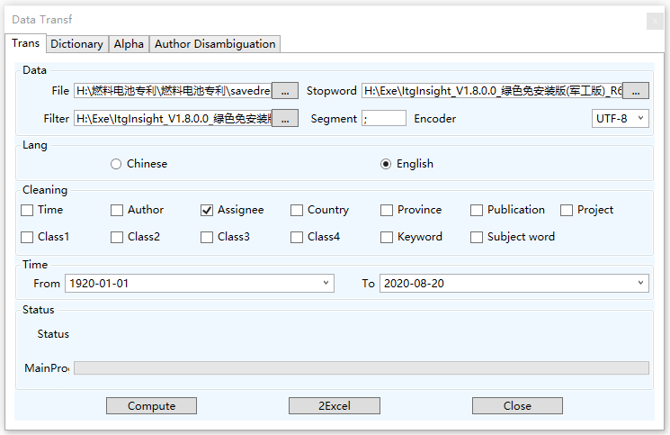
Next, switch to the “Dictionary/Thesaurus” tab, and select the appropriate dictionary (usually the default dictionary located in the “dic” directory of the installation folder). Additionally, users can choose the “Apply Thesaurus/Application Vocabulary” option for word segmentation, as shown below:

Switch to the Alpha/Thresholds tab as shown below:
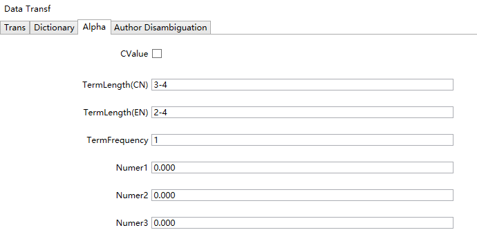
The C-Value method is a term calculation approach that can take a significant amount of time to compute, but can provide a valuable reference for identifying relevant terms. Users can adjust the choice of word length and frequency based on their preferences. For larger datasets, it is recommended to set more generous threshold values. Keyword merging can be performed using the “UpdateGroup_Auto” function (see Section 6.4: Data Auto-Grouping for Data Cleaning).
Chapter 10: Interacting with VosViewer, Pajek, Ucinet
The system supports exporting visual graphics to input format files of visualization software such as VosViewer, Pajek, and Ucinet. To save the file, users can simply click “Save” as shown below:
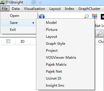
The saved file can then be directly used by VosViewer, Pajek, or Ucinet. Additionally, the system provides a graphic file in Pajek software net format, as illustrated below. Users can click to open the file and select the corresponding net file:
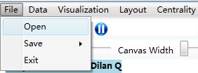
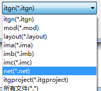
This software also supports graphic file input in netx format with the “.netx” extension. One key difference between netx and net format is that netx allows users to specify the size of network nodes. For more details on the specific format, please refer to the example/netx/example.netx file.
Chapter 11: Automatic Reporting
ITGInsight utilizes machine learning to automate, optimize, and modularize research reports. The system provides default report writing templates, and users can also customize report templates. The automatic report function is available to top-level enterprise users only. The intelligent organization of reports is performed by computers, and users are only required to make minor modifications. The following steps illustrate how to create an automatic report:
Open the .itgn file and click on the word icon in the menu bar. This will open a dialogue box where you can select the type of report you wish to generate.

The system supports three types of templates: theme analysis templates, single agency evaluation templates, and multiple agency comparison templates.Select the report template you want to use, and fill in the technical field of the analysis report in the Topic/theme text box, for instance, “nanotechnology.”Click the OK/OK button, and the software will automatically generate the report. Users can modify the report as needed. You can refer to the video tutorial for details on intelligent report writing. The intermediate results of the report, including various vector diagrams and statistical tables, are stored in the software installation directory report temple.
\ 
12.1 Metadata Import and Export
Metadata refers to the one-to-one correspondence between the graphic data and the data imported after the completion of data analysis and graphic drawing. It is similar to the incremental column function of GELPHI. The specific steps to use metadata are as follows:
After drawing any graphics, you can click the Metadata button on the toolbar to access the metadata page.
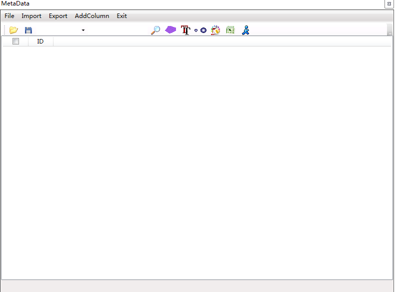
From there, you can import metadata in Access, Excel, or TXT format. The TXT format metadata file should be formatted as follows:
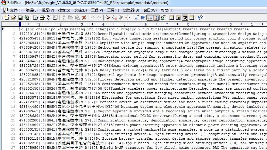
The first row contains the headers, followed by data columns separated by “|”. The metadata and graphic data are matched using the ID column, which must be a numeric format (e.g., 1, 2, 3, 4, etc.). If the imported metadata does not include the ID column, the software will automatically add one. The ID column requirements for EXCEL and ACCESS formats are the same.
To import metadata columns as numerical data, add “/double” to the header. For instance, if the column “ipc_chars” is to be imported as numeric data, set the header to “ipc_chars/double”.
It is recommended to import metadata in Excel format.
If the original metadata needs to be exported, click the Export button to export the metadata in TXT format by default. To export metadata in Excel format, click the Excel icon on the toolbar.
After importing the metadata, if you want to add a column, click the “Add Column” button. The import method is the same as importing metadata, you just need to add the column after the previously imported metadata.
12.3 Finding graphics based on metadata, changing node size, changing node text, drawing convex hull
Based on the imported metadata, the graph can be operated by selecting the column name of the operation from the toolbar ![]() , as shown below. Use the toolbar to modify the graphics by adjusting the node size, changing the node text, and drawing the convex hull.
, as shown below. Use the toolbar to modify the graphics by adjusting the node size, changing the node text, and drawing the convex hull.
After importing the metadata, click on the “Save” button to prompt the software to save the metadata in .metadata format, which is a binary metadata format that can be opened directly later, saving the time of importing metadata each time.
Chapter 13: Converting to References
13.1 Export literature to WORD in bibliographic format
To export literature in bibliographic format to Word, click “Data/Data->Analysis/Analysis” on the menu bar to bring up the data conversion page. Click “ToReference” to convert the bibliographic item into a Word document in reference format. It’s important to note that the selected filter must be in the filter directory, marked as a special filter for “ToReference,” as shown in the figure below: 
The reference format editor can be found in the Referenceformat.json file in the software directory. To open it, follow these steps:

According to the value of “PublicationType” in the filter, if the field value of “PublicationType” in the document is “J”, the reference format is used for reference editing. The symbols used in the format have the following meanings:
AuthorMeta$: When outputting references, the authors of the literature are separated by commas.
+.$AuthorMeta: If there is a document author field, add the symbol “.” after the author.
You can customize the reference format according to your needs. The software supports the conversion of bibliographic items from CNKI and SCI into references by default and also allows you to add reference formats of other data sources.
Appendix A. Co-author/co-occurrence/coupling
| Model\graphic element | Node size | Node color | Node connection | Node text |
| Number of first, second and third authors | Number of first authors in red, number of second authors in green, and number of third authors in yellow. | The thickness of the lines in the coherent/co-occurrence/couplings visualization represents the number of connections between the nodes. If the VS or UP layout algorithms are selected, the length of the connection is inversely proportional to the number of connections it represents. | Author / Agency / Country / Publication | |

|
Quantity | The color gradient gradually fades from the center to the edge of the ring, with the color intensity representing the number of years, and the red color indicating the closest proximity to the current time. | Ibid. | Ibid. |

| Model\graphic element | Node size | Node color | Node connection | Node text |
| Quantity | Meaningless | The thicker the line, the stronger the correlation; conversely, the thinner the line (if the VS and UP layout algorithms are selected, the length of the connection is inversely proportional to the number represented by the connection). | Author/institution/country/age | |

|
Ibid. | The color gradient goes from dark to light from the inside to the outside, and the color ring size is proportional to the number of occurrences in each year. Red represents the most recent year closest to the present time. | Ibid. | Ibid. |

| Model\graphic element | Node size | Node color | Node shape | Node connection | Node text |
| Quantity | Meaningless | A circle represents an author or organization, while a rectangle represents a technology category. | The thickness of the line connecting two nodes represents the strength of their correlation. Thicker lines indicate higher correlation, while thinner lines indicate lower correlation. If the VS and UP layout algorithms are chosen, the length of the connection is inversely proportional to the number represented by the connection. | Author/institution/country/age/category |
Appendix D. Citation relationship
| Model\graphic element | Node size | Node color | Node connection | Node connection |
| Literature citation | Meaningless | Meaningless | Citation relationship | Document number
(primary key literature) |
| Author/institution/Journal citation | Quoted quantity | Meaningless | Citation relationship | Author + age /
Institution + age / Publication + age |